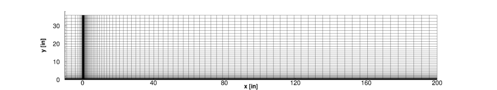
Figure 1a. Mach 0.2 Flat Plate ("structured") grid
This case examines the boundary layer formation of a Mach 0.2 flow along a flat plate. Skin friction and y+ plots of the boundary layer were studied in this case. This case is analogous to that used for the structured grid flat plate validation.
| Mach | Pressure (psia) | Temperature (R) | Angle-of-Attack (deg) | Angle-of-Sideslip (deg) |
|---|---|---|---|---|
| 0.2 | 14.7 | 530.0 | 0.0 | 0.0 |
| Wind-US 3.150 |
|---|
| fp0p2.tar |
In Figure 1a, the same structured grid as that used for the structured grid validation is shown. The grid has 111 points in the axial direction and 81 points in the vertical direction. The grid was packed to the wall such that the first point corresponded to a y+ value of 1 or less. Note the y+ spacing study shown on the structured grid flat plate boundary layer test case page. For use with the unstructured solver, the individuals cells are hexahedrals. In the rest of the discussion on this webpage, "structured" grid refers to this hexahedral grid that indeed looks structured but is in fact saved in unstructured hexahedral cell format. In Figure 1b and 1c, a modified grid is used where the first 51 points away from the wall are retained as the original "structured" hexahedral cells, and then away from this region, the cells are triangular prisms. The entire grid is one cell wide in the z-direction.
The grids shown in Table 3 are all in unstructured format. The "structured" grid simply refers to the fact that the topology is exactly the same as that of the structured case. The "unstructured" grid combines hexahedral cells near the wall and triangular prisms away from the wall, as discussed above.
Figure 1a. Mach 0.2 Flat Plate ("structured") grid
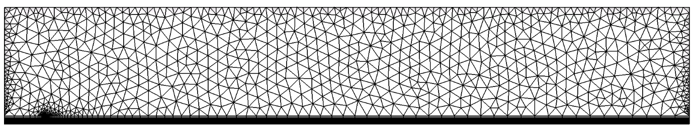
Figure 1b. Mach 0.2 Flat Plate (unstructured) grid
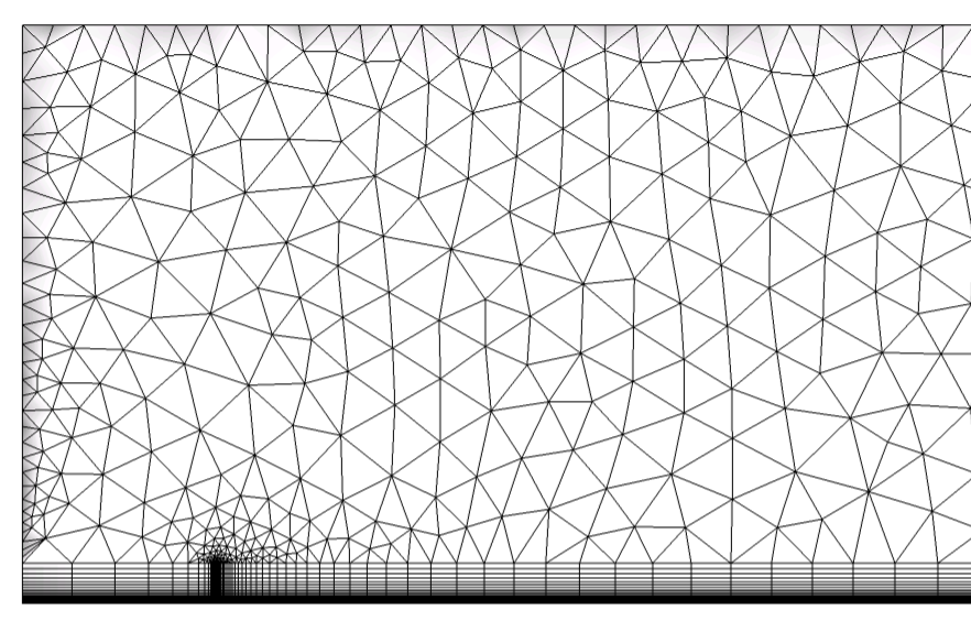
Figure 1c. Mach 0.2 Flat Plate (unstructured) grid (zoom)
| Common Grid ("Structured") | Common Grid (Unstructured) | Gridgen ("Structured") | Gridgen (Unstructured) | |
|---|---|---|---|---|
| File | fp_uns_1.cgd | fp_uns_2.cgd | fp_uns_1.gg | fp_uns_2.gg |
Boundary conditions for this flat plate case are as shown in Figure 2. Note that the first 14 points along the bottom are set to inviscid, such that the leading edge of the plate is at grid point 15 in the axial direction along the bottom of the grid. Although only the hexahedral or "structured" grid is shown in the figure, the boundary conditions are the same for the other grid, having triangular prisms away from the wall.
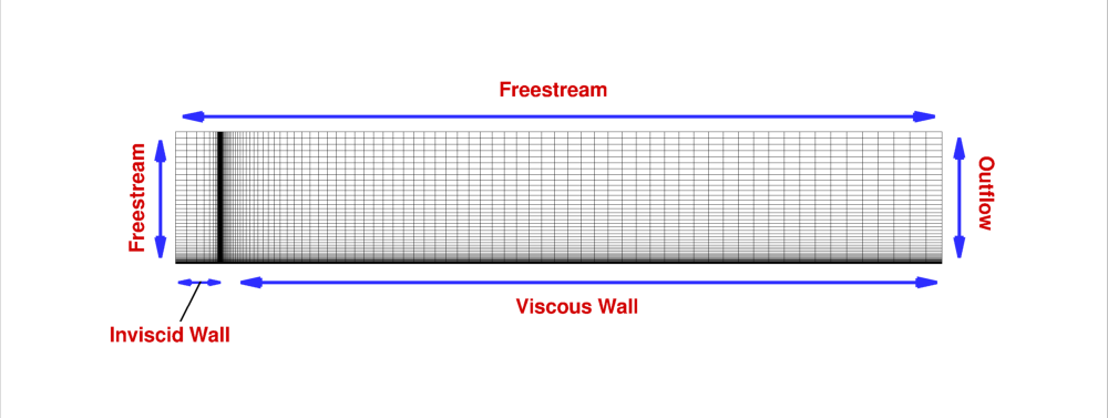
Figure 2. Boundary conditions.
Monitoring the residuals and key flow field quantities, for this case the wall skin friction coefficient, were the methods of determining convergence of this case. Below are the algorithm settings used in the dat file for these unstructured solver cases. Note that settings for the structured solver (i.e. choice of RHS method) were different, and may be found on the structured solver page for this flat plate case.
| Field | Spalart-Allmaras Structured Grid with Unstructured Solver | SST Structured Grid with Unstructured Solver | Spalart-Allmaras Unstructured Grid with Unstructured Solver | SST Unstructured Grid with Unstructured Solver |
|---|---|---|---|---|
| Version | Wind-US 3.150 | Wind-US 3.150 | Wind-US 3.150 | Wind-US 3.150 |
| Cycles | 5000 cycles | 5000 cycles | 5000 cycles | 5000 cycles |
| Convergence Order | 10 | 10 | 10 | 10 |
| Method | IMPLICIT UGAUSS LINE EXACT_LHS VISCOUS JACOBIAN FULL CONVERGE FREQUENCY 11 SUBITERATIONS 6 | IMPLICIT UGAUSS LINE EXACT_LHS VISCOUS JACOBIAN FULL CONVERGE FREQUENCY 11 SUBITERATIONS 6 | IMPLICIT UGAUSS LINE EXACT_LHS VISCOUS JACOBIAN FULL CONVERGE FREQUENCY 11 SUBITERATIONS 6 | IMPLICIT UGAUSS LINE EXACT_LHS VISCOUS JACOBIAN FULL CONVERGE FREQUENCY 11 SUBITERATIONS 6 |
| CFL | AUTO DECREASE 2 CFLMAX 100000 | AUTO DECREASE 2 CFLMAX 100000 | AUTO DECREASE 2 CFLMAX 100000 | AUTO DECREASE 2 CFLMAX 100000 |
| Limiters | DQ LIMITER ON RELAX 0.1 | DQ LIMITER ON RELAX 0.1 | DQ LIMITER ON RELAX 0.1 | DQ LIMITER ON RELAX 0.1 |
| Dissipation | TVD BARTH 3.0 | TVD BARTH 3.0 | TVD BARTH 3.0 | TVD BARTH 3.0 |
| Boundaries | IMPLICIT BOUNDARY ON | IMPLICIT BOUNDARY ON | IMPLICIT BOUNDARY ON | IMPLICIT BOUNDARY ON |
| RHS | HLLE SECOND | HLLE SECOND | HLLE SECOND | HLLE SECOND |
| Gradients | LEAST_SQUARES | LEAST_SQUARES | LEAST_SQUARES | LEAST_SQUARES |
| Turbulence | SPALART | SST | SPALART | SST |
| cfpart - to create lines | Spalart-Allmaras | SST |
|---|---|---|
| fp_cfpart.inp | sa.dat | sst.dat |
The post-processing files needed for this case are shown in Table 6.
| Hexahedral "structured" Post-processing FORTRAN code |
Hexahedral / triangular prism "unstructured" Post-processing FORTRAN code |
Velocity | Skin Friction Coefficient | Directions |
|---|---|---|---|---|
| POST.f | POSTus.f | vel.com | cf.com | README |
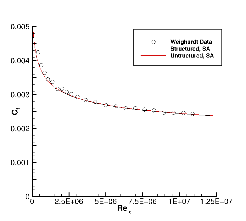
Figure 3. Spalart-Allmaras skin friction coefficient
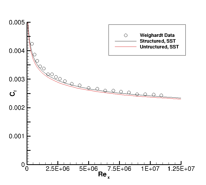
Figure 4. SST skin friction coefficient
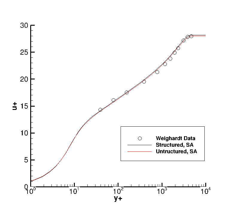
Figure 6. Spalart-Allmaras velocity profile
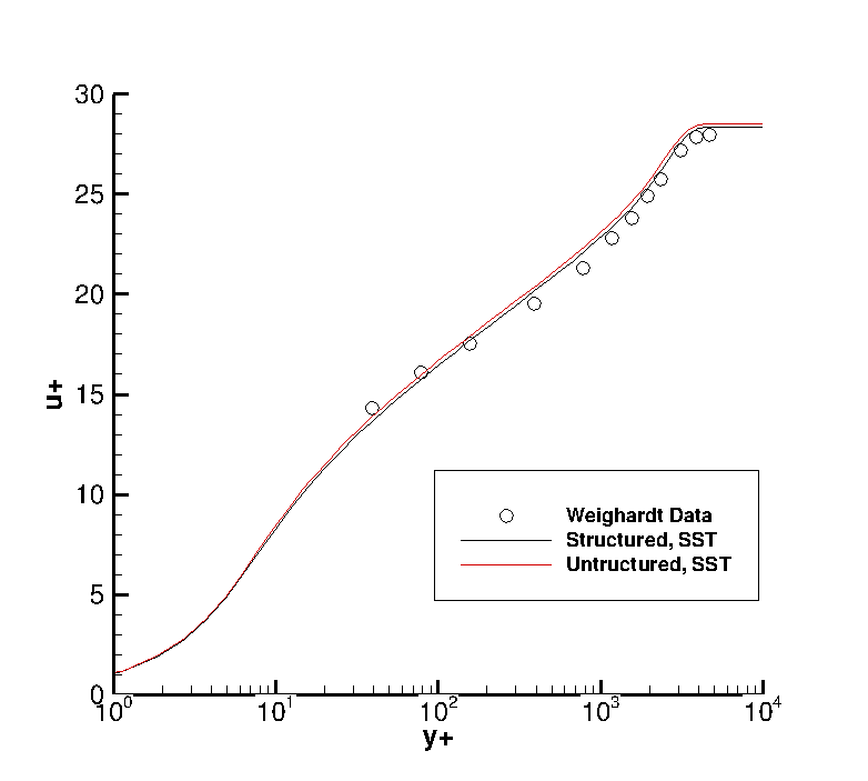
Figure 7. SST velocity profile
This validation test case was performed by Nick Georgiadis, Keven Lenahan, and Manan Vyas. Contact: Nick Georgiadis, (216) 433-3958 or Manan Vyas, (216) 433-6053, MS 5-12, NASA Glenn Research Center, 21000 Brook Park Road, Cleveland, Ohio, 44135.