Figure 1. Pressure contours on the surface and
symmetry plane of the ONERA M6 wing.
Figure 1. Pressure contours on the surface and
symmetry plane of the ONERA M6 wing.
This study is an example study demonstrating the application of the WIND code for solving the three-dimensional, transonic, turbulent flow over the ONERA M6 wing.
Most of the files for this example study are available in the Unix compressed tar file m6wing01.tar.Z. The files can then be extracted by the unix command:
uncompress -c m6wing01.tar.Z | tar xvof -
The files m6wing.x.fmt, run.cgd, run.cfl, run.lis along with some graphics files are not included in order to limit the size of the tar file. They can be downloaded separately.
The grid is contained in a PLOT3D grid file (formatted, multi-zone, whole, three-dimensional) named m6wing.x.fmt. It consists of four zones wrapped as a C-grid about the wing leading edge. Table 1 lists the zones and dimensions. The grid consists of a total of 316932 grid points.
| Zone | Dimension | Total Grid Points |
|---|---|---|
| 1 | 25 x 49 x 33 | 40425 |
| 2 | 73 x 49 x 33 | 118041 |
| 3 | 73 x 49 x 33 | 118041 |
| 4 | 25 x 49 x 33 | 40425 |
The J1 surface of zone 2 contains the lower surface of the wing and the J1 surface of zone 3 contains the upper surface of the wing. The K1 surfaces of all the zones are on the symmetry plane. The KMAX boundaries are coupled to eachother as they envelope the wing tip. The I1 surface of zone 1 and the IMAX surface of zone 4 are the outflow boundaries. The JMAX surfaces of all the zones are on the farfield boundary. The remaining zone boundaries are coupled to other zone boundaries. Figure 2 shows the surfaces of the wing, outlines of the zones, and the grids on the symmetry (K1) planes. Figure 3 shows the grid about the tip of the wing. The grid is clustered about the wing surface to resolve the boundary layer. However, the spacing of the grid normal to the wing surface is approximately 5.0E-05 feet, which will only resolve the turbulent boundary layer with the first grid point off the wall of y+ of approximately 30. Thus, the wall function will be used with this grid.
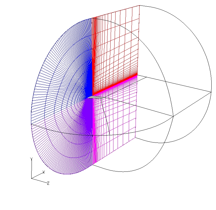
Figure 2. Surfaces, zones and grids for the ONERA M6 wing.
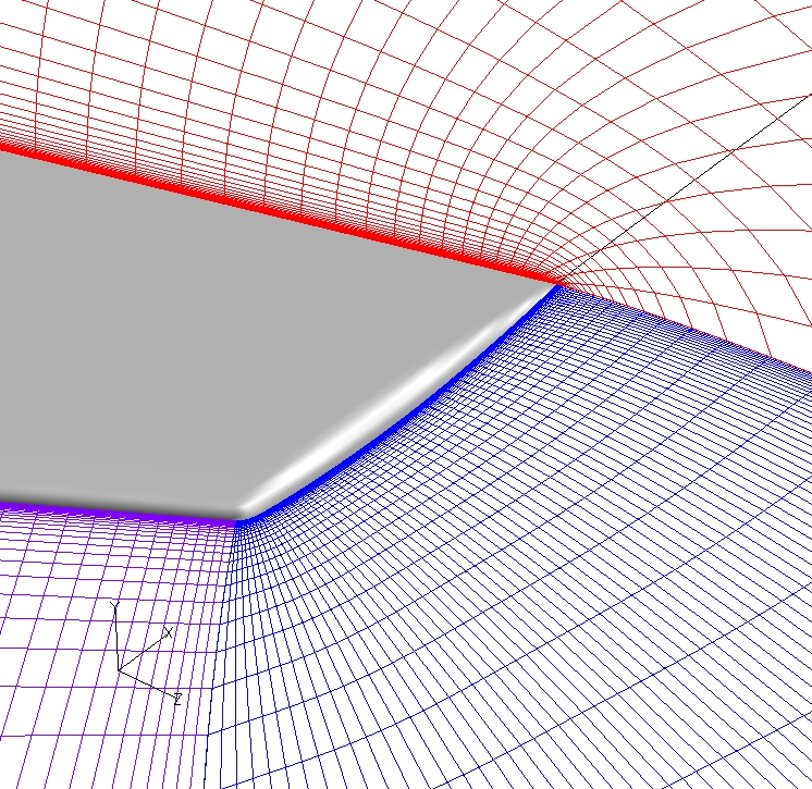
Figure 3. Grid near the tip of the wing.
The Plot3d grid file is converted to the common grid file (*.cgd) format using the CFCNVT utility. This is done using the command:
cfcnvt < cfcnvt.x.com
where the file cfcnvt.x.com is a command input file directed to the standard Fortran input unit. A common grid file named run.cgd is created.
The boundaries at the surface of the wing are specified as VISCOUS WALL boundary conditions. The boundaries at the symmetry plane are specified as REFLECTION boundary conditions, which is equivalent to an INVISCID WALL boundary condition. The boundaries at the outflow are specified as OUTFLOW boundary conditions even though the flow is not truly confined. This boundary condition allows the pressure to be specified, which is set to the freestream pressure. The boundaries at the farfield are specified as FREESTREAM boundary conditions, which uses one-dimensional characteristic theory to set conditions. The remaining boundaries are COUPLED to other zone boundaries.
The boundary conditions are set within the common grid file run.cgd by using GMAN. GMAN can be executed using either a) an interactive graphics interface or b) in a batch processing mode. The interactive mode is illustrated using step-by-step instructions. The batch processing mode is described below.
As GMAN operates, a journal file gman.jou is created which can later be used as a command file to re-run GMAN in batch mode. Here this file has been renamed gman.a.com and GMAN can be re-run as:
gman < gman.a.com
where the file gman.a.com is a command input file (standard Fortran input unit). The commond grid file run.cgd is updated in the process. In examining the file gman.a.com, one can see that one sets boundary conditions by specifying the surface and then the boundary condition type.
An alternative to directly specifying the coupling between zone is to use the automatic coupling method in GMAN. This can be done prior to setting the boundary conditions. The procedure is:
Pick BOUNDARY COND. (left panel)
Pick AUTO COUPLE
Pick RUN AUTO COUP
GMAN will then search through each zone boundary and check to see if there are any other zone boundaries that are coincident. Note that this may take a significant amount of time if there are a large number of zones and the grid is large. It is suggested that one set the physical boundary conditions (i.e. viscous wall, freestream, etc...) prior to starting the automatic coupling search. Also note that automatic coupling will not detect a self-coupled boundary.
The command file to use the automatic coupling is gman.b.com and GMAN can be re-run as:
gman < gman.b.com
Upon completion of the batch operation, one should see the line "Congratulations, no undefined points left", which indicates that all boundary grid points have been assigned a boundary condition type or have been coupled to other boundary grid points.
The computation is performed using the time-marching capabilities of WIND to march to a steady-state (time asymptotic) solution starting from an initial solution. Local time stepping is used at each iteration to enhance iterative convergence. The flow is assumed to be fully turbulent.
The initial flow conditions are the freestream flow values as presented in Table 2. These corresond to a Reynolds number of 11.72 million based on the mean aerodynamic chord length. These conditions match the Mach number, Reynolds number, and angle-of-attack of test 2308 from the paper by Schmitt and Charpin in AGARD Report AR-138 referenced below. The static temperature was selected to be 460 degrees Rankine, which with the Mach and Reynolds number yielded a static pressure of 45.82899 psi.
| Mach | Pressure (psia) | Temperature (R) | Angle-of-Attack (deg) | Angle-of-Sideslip (deg) |
|---|---|---|---|---|
| 0.8395 | 45.82899 | 460.0 | 3.06 | 0.0 |
The WIND input data file for this case is run.dat. The first three lines describe the flow problem. The freestream keyword indicates that the static freestream flow conditions are specified as Mach number, pressure (psia), temperature (R), angle-of-attack (degrees), and angle-of-sideslip (degrees). The turbulence model keyword indicates that the Spalart-Allmaras turbulence model is to be used. The wall function keyword indicates that the wall function is used since the spacing of the first grid point off the wall will only yield a y+ value of approximately 30. The implicit boundary keyword indicates that implicit boundary conditions are used at the viscous wall boundaries. The dq limiter keyword indicates that changes in density and temperature over an iteration are limited to 50% of the current value at each solution point. The downstream pressure keyword indicates that the freestream pressure is imposed on the outflow boundaries specified with a OUTFLOW bounary condition. The loads keyword indicates that the forces on the wing are to be integrated every 20 iterations and displayed in the output list file. This will we used to evaluate the convergence of the solution. The cycles keyword indicates that a maximum of 1000 cycles will be run. The iterations per cycle keyword indicates that 5 iterations will be run per cycle and that convergence information will be written to the output list file every 5 iterations. The cfl keyword indicates that a CFL number of 2.5 will be used. By default, WIND uses local maximum allowable time-step based on the specified CFL number. The converge order keyword indicates that the computation will stop if the L2 norm of the solution drops by 9 orders-of-magnitude.
The WIND solver is run on a UNIX computer by entering the command:
wind -runinplace -dat run -mp -parallel
This runs the wind script which sets up the computation for the solver. Further details and options for the wind script can be found in the WIND documentation (wind script). A brief description of script options can be listed by typing:
wind -help
The -runinplace option indicates that WIND is to be run in the directory in which the wind script is executed. Otherwise a temporary directory is created for the computation.
The -dat run option indicates that the input data file run.dat has the prefix run.
The -mp option indicates that the computation is being performed on a multi-processor computer. The -parallel option is used along with the -mp option to indicate that the computation will be executed in parallel. The parallel computing capability also requires the creation of a multiple processor control file named run.mpc that includes information on how many processors to use.
To run WIND on one processor in serial mode, just use:
wind -runinplace -dat run
Some interactive prompts ask for information to finish setting up the computation:
First, one is asked to select the version of WIND that will be used. Hitting a "return" will default to selecting the latest production version of WIND. There may be "alpha" or "beta" versions listed that are currently under development and being tested.
The next three prompts ask for the names of the output list file (run.lis), mesh file (run.cgd), and flow data file (run.cfl). Hitting Return will default to using the prefix of the -dat option. If a flow data file with the specified name exists, the computation will start from that solution. Otherwise, a solution will be initialized with the freestream conditions. The wind script will indicate whether an existing solution file has been found.
The next question allows a choice between running the solution in real-time (interactive) or submitting it to a queue.
Running Real-Time. Running the computation in real-time will give the computation a higher priority on the computer if several jobs are already running. The next questions asks whether the output should be written to the screen. Enter n so that screen output is written to a list file named run.lis. A "return" will cause the job to be submitted and the computation begun.
Running in Batch. On an SGI workstation, a batch job will be submitted to the AT queue. The job may run with other jobs in the queue, but may have lower priority. The defaults may be chosen for the remaining prompts. The options exist to specify the start and end times of the computation. A "return" will cause the job to be submitted and the computation begun.
The output list file is run.lis and contains the output from the computation and lists the residual information for both the flow equations and the turbulence model equation for each iteration. The integrated forces for the top portion of the wing is also output every 10 iterations. When running parallel, the list file also reports the multi-processor performance statistics.
The flow data file is run.cfl and contains the final solution.
After running the computation, one must then demonstrate iterative convergence of the steady-state solution. There are several ways to examine the iterative convergence:
Residual of the Navier-Stokes Equations. The L2 norm of the residual of the Navier-Stokes equations can be read from the output list file run.lis. The RESPLT utility is used in the form,
resplt < resplt.nsl2.com
The file resplt.nsl2.com is a command file containing the inputs for RESPLT to output the GENPLOT formatted plot data file named nsl2.gen of the residuals as a function of the number of iterations. This file can be plotted using CFPOST,
cfpost < cfpost.nsl2.com
where the file cfpost.nsl2.com is a command file containing the inputs for CFPOST. Figure 4 shows the solution residual that is displayed by CFPOST.
Figure 4. Plot of the L2 norm of Navier-Stokes residuals.
Residual of the Spalart-Allmaras Turbulence Model. The L2 norm of the residual of the governing equation used in the Spalart-Allmaras turbulence model can be read from the output list file run.lis. The RESPLT utility is used in the form
resplt < resplt.sal2.com
The file resplt.sal2.com is a command file containing the inputs for RESPLT to output the GENPLOT formatted plot data file named sal2.gen of the residual as a function of the number of iterations. This file can be plotted using CFPOST,
cfpost < cfpost.sal2.com
where the file cfpost.sal2.com is a command file containing the inputs for CFPOST. Figure 5 shows the solution residual that is displayed by CFPOST.
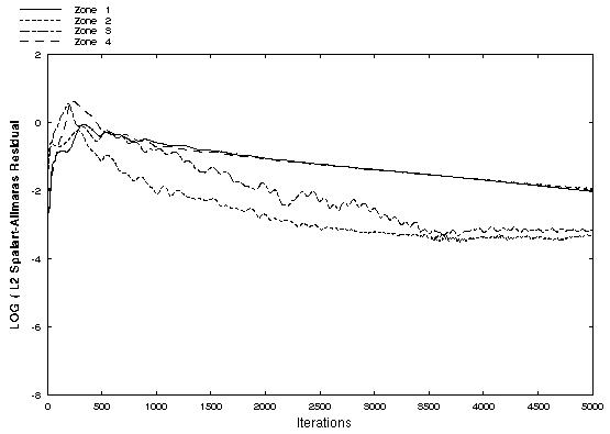
Figure 5. Plot of the L2 norm of the Spalart-Allmaras
turbulence equation residuals.
Wing Lift and Drag. Since determining the lift and drag of the wing is a primary engineering objective. One can monitor the change of these values with iterations and determine the point of iterative convergence when these values no longer significantly change. The loads keyword in the input data file run.dat outputs this information into the output list file run.lis. RESPLT is then used to read this information and create plot files,
resplt < resplt.liftconv.com
The file resplt.liftconv.com is a command file containing the inputs for RESPLT to output the GENPLOT formatted plot data file named liftconv.gen of the residuals as a function of the iterations. This file can be plotted using CFPOST,
cfpost < cfpost.liftconv.com
where the file cfpost.liftconv.com is a command file containing the inputs for CFPOST. CFPOST will display in sequence the plots for drag, lift, and z-direction force. Figures 6 and 7 show the convergence of the drag and lift as displayed by CFPOST.
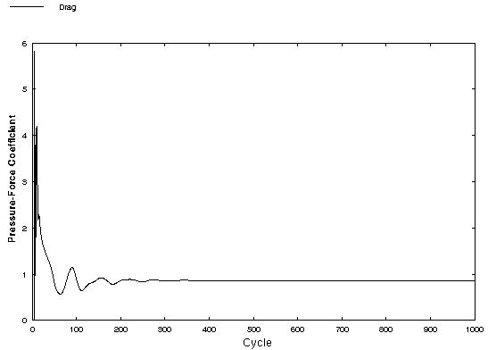
Figure 6. Plot of the drag of the
ONERA M6 wing with respect to the number of iterations.
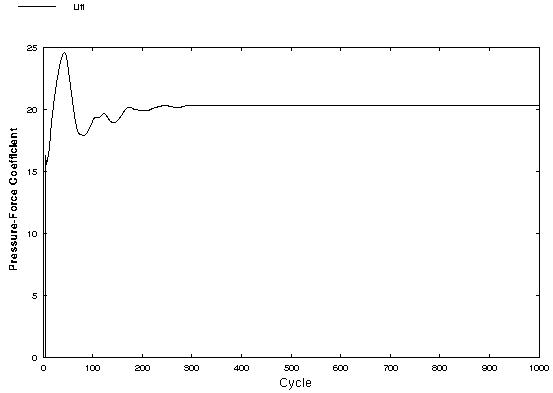
Figure 7. Plot of the lift of the
ONERA M6 wing with respect to the number of iterations.
The CFPOST utility can be used to generate engineering information from the the data files.
PLOT3D Grid and Solution Files. The PLOT3D grid and solution files can be obtained for use in commercial visualization software (i.e. Fieldview, Ensight, Tecplot) using the commands:
cfpost < cfpost.plot3d.com
The PLOT3D grid and solution files are named run.x and run.q, respectively. They are unformatted, whole, 3D, and multi-zone.
Mach Number Contour Plots. The CFPOST utility can be used to generate and plot flow contours at a cutting plane perpendicular to the wing span. Here the Mach number contours are generated and plotted at section 1 (y/b=0.2),
cfpost < cfpost.zcut.mach.com
Pressure Coefficient Distribution. The referenced experiment (Schmitt and Charpin, 1979) obtained pressure coefficients at seven sections along the span of the wing. Corresponding pressure coefficients can be obtained from the WIND flow solution using CFPOST,
cfpost < cfpost.zcut.cp1.com
where cfpost.zcut.cp1.com is the command input file for CFPOST to obtain the pressure coefficient at section 1. A GENPLOT file named cp1.gen is created and plotted. The pressure coefficient is negative for pressures less than freestream, which occurs on the top of the wing. In plots of pressure coefficients for wings, the negative of the pressure coefficient is usually plotted to indicate that the lower pressure region is on the top of the wing and the high pressure region is on the bottom of the wing. This is done in the CFPOST command files. The data from the experiment is expressed with respect to the local chord length. A short Fortran 77 program, readgen.f, was written to transform the data in the GENPLOT file to be consistent with the format used in the experimental data. Figures 8 to 14 show the pressure coefficients at each section along the wing.
| Section | CFPOST Command File | GENPLOT File | Plot File |
|---|---|---|---|
| 1 | cfpost.zcut.cp1.com | cp1.gen | cp1.do |
| 2 | cfpost.zcut.cp2.com | cp2.gen | cp2.do |
| 3 | cfpost.zcut.cp3.com | cp3.gen | cp3.do |
| 4 | cfpost.zcut.cp4.com | cp4.gen | cp4.do |
| 5 | cfpost.zcut.cp5.com | cp5.gen | cp5.do |
| 6 | cfpost.zcut.cp6.com | cp6.gen | cp6.do |
| 7 | cfpost.zcut.cp7.com | cp7.gen | cp7.do |
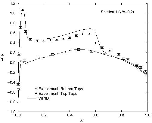
Figure 8. Plot of the pressure coefficients
on the wing surface at section 1 (y/b=0.20).
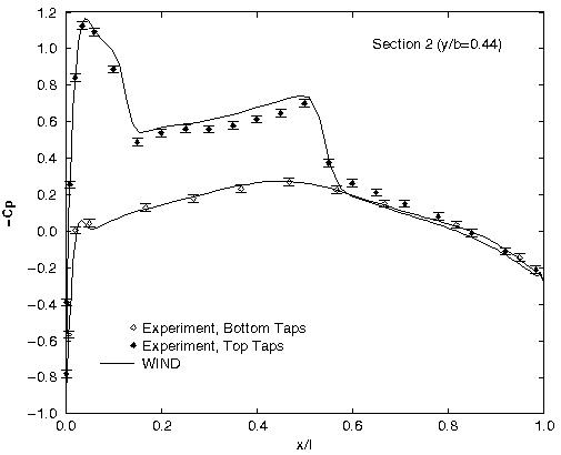
Figure 9. Plot of the pressure coefficients
on the wing surface at section 2 (y/b=0.44).
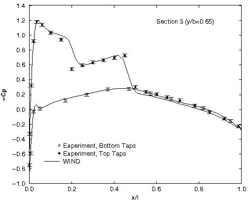
Figure 10. Plot of the pressure coefficients
on the wing surface at section 3 (y/b=0.65).
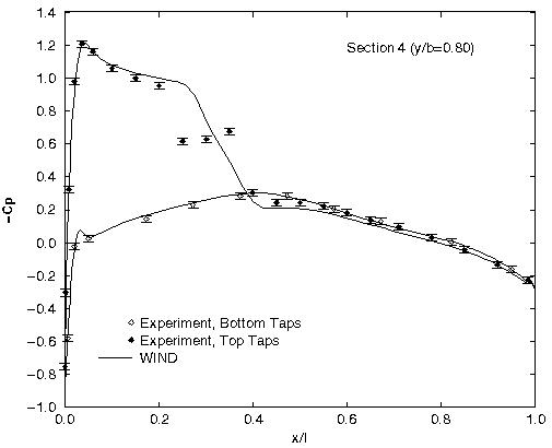
Figure 11. Plot of the pressure coefficients
on the wing surface at section 4 (y/b=0.80).
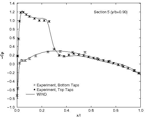
Figure 12. Plot of the pressure coefficients
on the wing surface at section 5 (y/b=0.90).
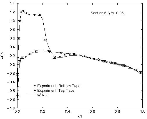
Figure 13. Plot of the pressure coefficients
on the wing surface at section 6 (y/b=0.95).
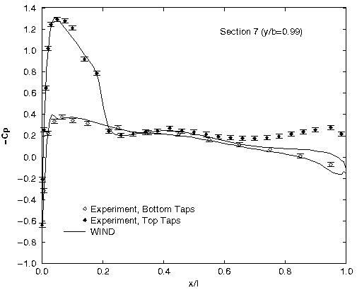
Figure 14. Plot of the pressure coefficients
on the wing surface at section 7 (y/b=0.99).
Forces on the Wing. For a wing calculation, another piece of important information is the forces on the wing which result from pressure and skin-friction. CFPOST can be used to integrate these forces over the surface of the wing,
cfpost < cfpost.forces.com
where cfpost.forces.com is the command input file for CFPOST. A list file named forces.lis is created in which the force information is printed.
Boundary Layer Properties. For a viscous computation, it is useful to examine how well the turbulent boundary layers were resolved. One measure of this is the y+ values at the grid points in the boundary layers. The forces list file forces.lis does contain a summary of the y+ values near the walls.
To examine the boundary layer at a certain location, CFPOST can be used,
cfpost < cfpost.blan.com
The file cfpost.blan.com is a command file which writes out the x and y coordinates, u-velocity, v-velocity, static temperature, and y+ values along a grid line at I60, which is on the top of the wing just before the trailing edge. This information is written to a GENPLOT file named blan.gen.
In examining the pressure coefficient comparisons of Figs. 8-14, one may conclude that the comparisons are good overall. It appears that there are two shocks on the upper surface at section 4 (y/b=0.80) which WIND does not capture. Determining the cause of differences between the computation and experiment requires sensitivity studies with respect to such things as the grid, turbulence model, and algorithms. Refining the resolution of the boundary layer to y+ of 1 may improve comparisons. Further streamwise refinement of the grid would help capture the shocks on the upper surface.
The computations were performed on a Silicon Graphics Octane II workstation using 2 600 MHZ IP30 MIPS R14000 Processors. 1000 cycles for 5000 iterations required ? CPU seconds over an elapsed time of ? seconds.
Schmitt, V. and F. Charpin, "Pressure Distributions on the ONERA-M6-Wing at Transonic Mach Numbers," Experimental Data Base for Computer Program Assessment. Report of the Fluid Dynamics Panel Working Group 04, AGARD AR 138, May 1979.
This study was last updated on August 30, 2002 by John W. Slater, who may be contacted at:
NASA John H. Glenn Research Center, MS 86-7
21000 Brookpark Road
Brook Park, Ohio 44135
Phone: (216) 433-8513
e-mail: John.W.Slater@grc.nasa.gov