
NPARC Alliance Validation Archive
Validation Home >
Archive >
S-Duct Inlet >
Study #3
In this study, use of the BAY vortex generator model is investigated for viscous flow in the M2129 circular S-duct with a throat Mach number of 0.78. The duct has vane-type vortex generators equally spaced in a co-rotating arrangement as shown in Fig. 1. The Wind-US code contains two vortex generator models, the Wendt model (Ref. 1) and the BAY model (Ref. 2). For an example of this S-duct computed using the Wendt model, see Study # 2.
All of the archive files of this validation case are available in the Unix compressed tar file sduct03.tar.gz. The files can then be accessed by the commands
gunzip sduct03.tar.gz
tar -xvof sduct03.tar
The geometry which was tested experimentally is test case 3 from the AGARD study of Ref. 3, and was referred to as the M2129 duct in the experimental investigations of Ref. 4. This duct has a circular cross section and an S-shaped centerline, and is shown in Fig. 1. The duct is approximately 2 ft (0.61 m) in length, and the throat, which is located at the end of the upstream straight section, is 5.06 in. (12.9 cm) in diameter. The engine face, or aerodynamic interface plane (AIP), is located at an axial station of 19.27 in (48.9 cm), it's diameter is 6.0 in. (15.2 cm), and the duct offset is 5.4 in. (13.7 cm).
The VG configuration tested is referred to as VG170 in Ref. 4 and contains 11 flat-plate vanes per half duct, located one inlet diameter downstream of the inlet throat. Each generator has a height-to-chord ratio of 0.25, where the chord is approximately 0.7 in. (1.8 cm), and an angle of incidence of 16 deg. This configuration was designed to turn the flow near the wall away from the bottom of the duct, and ideally counteract the formation of the duct vortex.
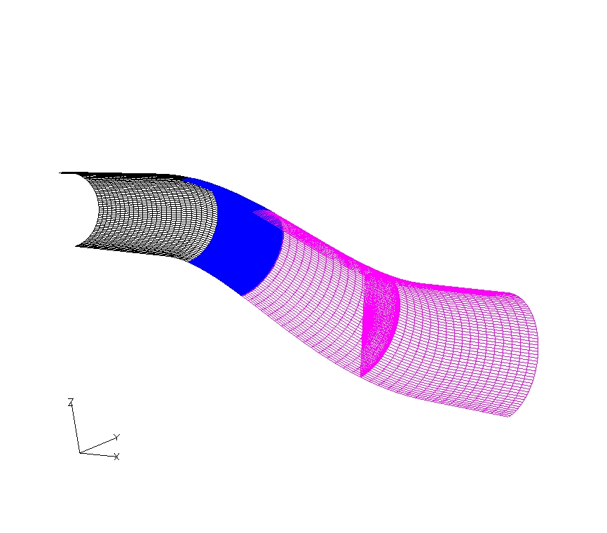
The computational grid used for this simulation is sduct03.cgd and it is shown in Fig. 2. Since the duct is symmetric about the x-z-plane, only half of the duct is gridded. The grid has three zones, and the vortex generator model is applied in ZONE 2, over the 11 individual grid regions containing each generator. The grid spacing in the vicinity of the generators as a percentage of the VG chord length is 0.26 in the axial direction, 0.64 in the radial direction and 0.54 in the circumferential direction. The grid has a total of 677,940 points as given below. The grid in the formatted, multi-block Plot3D format is available in the file sduct03.x.fmt.
| ZONE | Dimensions (psia) |
|---|---|
| 1 | 26x61x49 |
| 2 | 36x277x50 |
| 3 | 34x61x49 |
An initial condition of freestream flow was used, as given in Table 2:
| Mach number | Total Pressure (psia) | Total Temperature(R) | Angle-of-Attack (deg) |
|---|---|---|---|
| 0.7 | 14.67 | 517.0 | 0.0 |
In all three blocks, the KMAX boundary is a VISCOUS WALL, the KMIN boundary is a SINGULAR AXIS, and the J1 and JMAX boundaries are set to REFLECTION. In ZONE 1, the I1 boundary is set to ARBITRARY INFLOW. In ZONE 3, the IMAX boundary is set to OUTFLOW. The zonal interfaces on the I-boundaries between zones are all coupled. The vortex generator model is addressed in the Input Parameters and Files section.
The boundary conditions are specified using GMAN. This was done using the command:
gman < gman.sduct03.com
where the file gman.sduct03.com is a command input file. This file instructs GMAN to read in the sduct03.cgd grid file, and to set all of the boundary conditions. This could also be done using GMAN's graphical mode. (For a good example case using GMAN's graphical mode, see the Laminar Flat Plate case.)
The computation is performed using the time-marching capabilities of WIND to approach the steady-state flow starting from the freestream conditions. Local time stepping is used at each grid point to speed up convergence. The flow is assumed to be fully turbulent. The first run establishes the baseline flow without the vortex generators. The BAY vortex generator model is then applied for the remaining iterations.
This case is computed in two runs. The first run is a baseline case run without the vortex generators. It's corresponding Wind-US input data file is sduct03.dat.1. The next run uses the BAY vortex generator model to specify 11 flat plate vanes, equally spaced about the circumference of the half-duct. It's corresponding input data file is sduct03.dat.2. The FREESTREAM keyword is used to specifiy the freestream conditions, which are given in Table 2, above. For ZONE 1, the ARBITRARY INFLOW keyword indicates that the total temperature and the local flow angles are held constant, and the inflow is uniform and matches the freestream conditions. The DOWNSTREAM PRESSURE keyword sets the outflow pressure in ZONE 3 to 12.63 psi. The TURBULENCE keyword indicates that the Spalart-Allmaras turbulence model is used. The CFL# keyword sets the initial CFL number to 0.15 for the first 500 iterations, then increments it by a factor of 1.5 every 100 iterations until it reaches a value of 2.0, where is then held constant. Both runs consist of 2000 cycles with 5 iterations per cycle for a total of 10000 iterations per run. The LOADS keyword is used to print out the mass flux at the I=34 of plane of ZONE 3 every 10 iterations. This is used to monitor convergence.
As mentioned above, the BAY vortex generator model is used in sduct03.dat.2 to specify the eleven vane vortex generators. All of the generators are in ZONE 2, and each has a chord length of 0.7 inches, height of 0.175 inches and an angle of incidence of -16 degrees. In this specific case, the grid is inclined 16 degrees in the vane region, so the angle of incidence of the model is specified as nearly 0, or -0.000001. The negative sign was needed in order to produce the correct rotation of the vortices since the leading edges of the vanes correspond to the maximum, rather than the minimum J indices specified by VANE_SPEC within the VORTEX GENERATOR model keyword. If case were to use a more typical baseline grid which is not aligned with the vanes, the angle of incidence of the model would be set to -16 degrees.
To run WIND-US, the input data file for the first run, sduct03.dat.1, was copied to sduct03.dat and the WIND-US job was run using the following command:
wind -dat sduct03 -grid sduct03Since the wind_post post processing script was located in the run directory; it automatically submitted run 2 immediately after run 1 was completed. The resulting solution files for each run are sduct03.cfl.1 and sduct03.cfl.2. The resulting output list file is sduct03.lis.
The RESPLT utility was used to obtain convergence history information from sduct03.lis. The following command was used to obtain the file chist.l2.gen, which contains the L2 residual in GENPLOT format.
resplt < resplt.1.com
Where the file resplt.1.com is a command input file. In the same manner, the command file resplt.2.com was used to create the GENPLOT file chist.mass.gen containing the mass flux history at the exit plane of ZONE 3. The plots of these results were created using the CFPOST postprocessing program and the files cfpost.1.com and cfpost.2.com as follows.
cfpost < cfpost.1.com
cfpost < cfpost.2.comThe resulting plots are shown in Fig. 3, below.
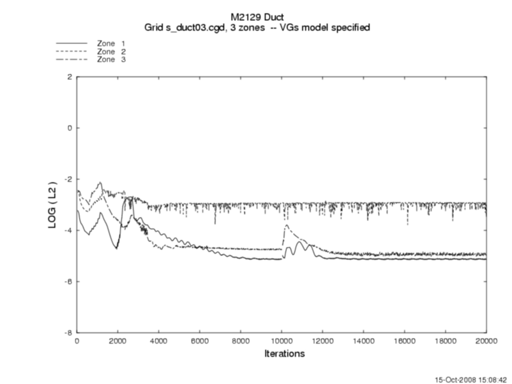
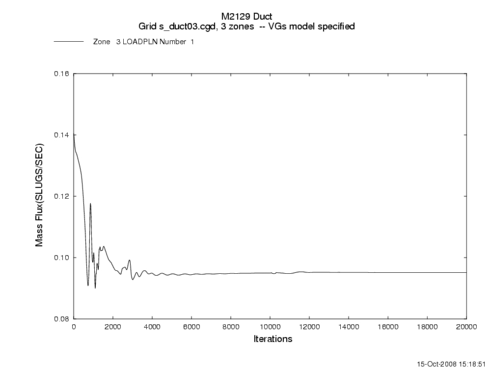
The L2 residuals oscillate at values near 10-3 for ZONE 2, and near 10-5 for ZONES 1 and 3, but do not show a big drop, as in the inviscid s-duct case of study 1, most likely due to the more complex and turbulent nature of this flow. The average mass flux at plane I = 34 in ZONE 3 is plotted in Figure 3 (b) and indicates that the mass flux has converged, and also that the use of the BAY vortex generator model, which is "turned on" at 10000 iterations, does not increase or decrease the mass flow. Rather than using the L2 residuals as the criteria for convergence, the convergence of the quantities of interest -- the total pressure recovery, the throat Mach number and the mass flux -- were used. This case was considered converged after approximately 20,000 iterations, at which point, the the total pressure recovery at the aerodynamic interface plane (AIP) converged to within four significant figures, and the throat Mach number to converged to three significant figures. Also, as shown in Fig. 3b, the mass flux has also converged.
Two quantities of interest in this duct are the area averaged total pressure recovery at the aerodynamic interface plane or AIP and the throat Mach number. To compute these quantities, which are given in Table 3 below, the CFPOST postprocessor was used with the command file cfpost.avg.com as follows.
cfpost < cfpost.avg.com
This produces two output files named cf.aip.2.lis and cf.thrt.2.lis, where the "2" corresponds to run number 2, which used the BAY vortex generator model to specify the VG effects. The results are tabulated in Table 3, along with the experimental result, a previous solution computed using gridded vanes and the results given in Study #2 which were computed using the Wendt vortex generator model. Based on Study #2 , the solutin is considered converged after 20,000 iterations since there is no appreciable change in the quantities of interest with further computation.
| Case | No. Iter. | AIP Total Pressure Recovery | Throat Mach Number |
|---|---|---|---|
| Experiment | |
|
|
| Gridded Vanes | 30000 | |
|
| Wendt Model | 20000 | |
|
| BAY Model | 20000 | |
|
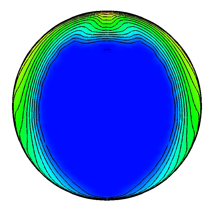
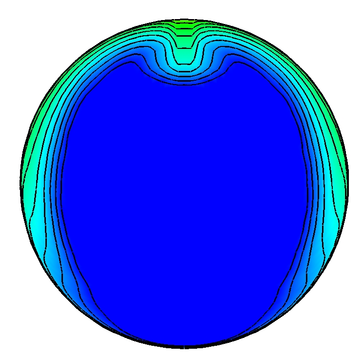
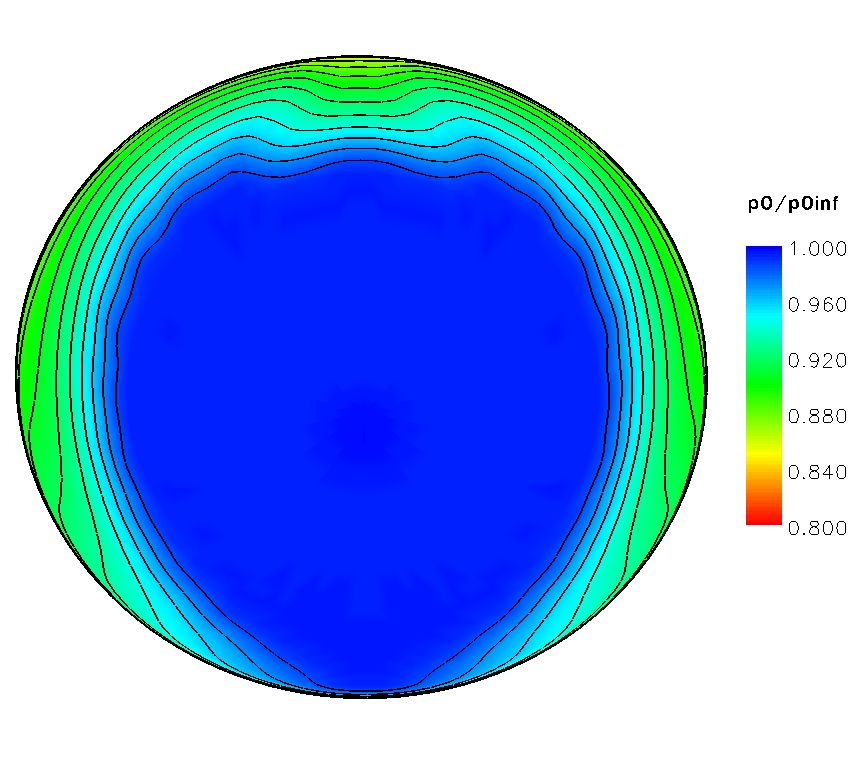
The total pressure at the duct AIP, located at an axial station of 19.3 inches, was plotted using the commercially available CFD postprocessing software Fieldview. The results of a previously computed gridded vane solution (See Ref. 4), the Wendt VG model, (see Study # 2) and the solution computed in this study using the BAY vortex generator model, are shown in Fig. 4, below.
a. | |
| | | | |
| | | | |
| |
b. |
| | | | |
| | | | |
c. |
|
|---|
These cases were run using WIND-US Alpha Version 3.25 on an HPXW9400 LINUX workstation. It took a total of 192,298 CPU seconds to run 20000 iterations or approximately 14.2 CPU sec/(iter-node). A nearly neglible increase in CPU time (approximately 1.2%) was observe when the BAY vortex generator model was used.
1. Dudek, J. C., "Empirical Model for Vane-Type Vortex Generators in an Navier-Stokes Code", AIAA Journal, Vol. 44, No. 8, pp 1779-1789, August 2006.
2. Bender, E. E., Anderson, B. H., and Yagle, P. J., "Vortex Generator Modeloing for Navier-Stokes Codes," Proceedings of the 3rd ASME/JSME Joint fluids Engineering Conerence, FEDSM99-6919, July 1999 .
3. "Air Intakes for High Speed Vehicles," AGARD-AR-270 (AGARD Advisory Report 270), Fluid Dynamics Panel Working Group 13, September 1991
4. Anderson, B. H., and Gibb, J., "Vortex Generator Installation Studies on Steady State and Dynamic Inlet Distortion," AIAA Paper 96-3279, July 1996.
This case was created on October 30, 2008 by Julianne C. Dudek, who may be contacted at
NASA Glenn Research Center, MS 5-12
21000 Brookpark Road
Cleveland, Ohio 44111
Phone: (216) 433-2188
e-mail: Julianne.C.Dudek@nasa.gov