
The steps involved in running the code are best shown by looking at some examples. The first example uses the default versions of subroutines COORS and POINTS to create a very simple plot, consisting of a two curves and a set of symbols. The second example also uses the default versions of subroutines COORS and POINTS, but is more complex, illustrating some of the capabilities of plotc. It plots the same curves and symbols as the first example, but includes a legend and a couple of text strings, uses two different fonts, has user-specified axis scales, and is in color. The third example is a simple illustration of the use of a user-written COORS routine.
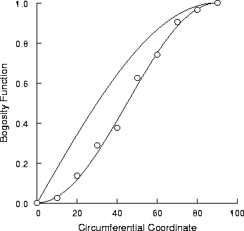
This example creates a very simple plot, consisting of a two curves and a set of symbols. Most of the namelist input is defaulted.
The namelist input file is listed below, along with explanatory notes for each line. Remember that with namelist input each line starts in column 2 or higher.
 &ptype
  ncurv=2, nsymb=1,                     Plot two curves and one set of symbols.
 &end
 &axes
 &end
Circumferential Coordinate              x-axis title.
Bogosity Function                       y-axis title.
Plotc Example 1                         Plot title.
    51                                  Curve 1 x and y coordinates.
       0.0       1.8       3.6       5.4       7.2       9.0      10.8      12.6
      14.4      16.2      18.0      19.8      21.6      23.4      25.2      27.0
      28.8      30.6      32.4      34.2      36.0      37.8      39.6      41.4
      43.2      45.0      46.8      48.6      50.4      52.2      54.0      55.8
      57.6      59.4      61.2      63.0      64.8      66.6      68.4      70.2
      72.0      73.8      75.6      77.4      79.2      81.0      82.8      84.6
      86.4      88.2      90.0
   0.00000   0.03141   0.06279   0.09411   0.12533   0.15643   0.18738   0.21814
   0.24869   0.27899   0.30902   0.33874   0.36812   0.39715   0.42578   0.45399
   0.48175   0.50904   0.53583   0.56208   0.58779   0.61291   0.63742   0.66131
   0.68455   0.70711   0.72897   0.75011   0.77051   0.79015   0.80902   0.82708
   0.84433   0.86074   0.87631   0.89101   0.90483   0.91775   0.92978   0.94088
   0.95106   0.96029   0.96858   0.97592   0.98229   0.98769   0.99211   0.99556
   0.99803   0.99951   1.00000
    51                                  Curve 2 x and y coordinates.
       0.0       1.8       3.6       5.4       7.2       9.0      10.8      12.6
      14.4      16.2      18.0      19.8      21.6      23.4      25.2      27.0
      28.8      30.6      32.4      34.2      36.0      37.8      39.6      41.4
      43.2      45.0      46.8      48.6      50.4      52.2      54.0      55.8
      57.6      59.4      61.2      63.0      64.8      66.6      68.4      70.2
      72.0      73.8      75.6      77.4      79.2      81.0      82.8      84.6
      86.4      88.2      90.0
   0.00000   0.00099   0.00394   0.00886   0.01571   0.02447   0.03511   0.04759
   0.06185   0.07784   0.09549   0.11474   0.13552   0.15773   0.18129   0.20611
   0.23209   0.25912   0.28711   0.31594   0.34549   0.37566   0.40631   0.43733
   0.46860   0.50000   0.53140   0.56267   0.59369   0.62434   0.65451   0.68406
   0.71289   0.74088   0.76791   0.79389   0.81871   0.84227   0.86448   0.88526
   0.90451   0.92216   0.93815   0.95241   0.96489   0.97553   0.98429   0.99114
   0.99606   0.99901   1.00000
   10                                   Symbol set 1 x and y coordinates.
        0.       10.       20.       30.       40.       50.       60.       70.
       80.       90.
   0.00000   0.02447   0.13552   0.28711   0.37566   0.62434   0.74088   0.90451
   0.96489   1.00000
The following terminal session shows how you would use the above input file to create your plot. Lines in slanted type are entered by the user. The remainder are printed by the computer. This example assumes the plotc namelist input file is bogus1.plotin.
plotc bogus1.plotin
Using namelist input file bogus1.plotin

PostScript output is in plotc.ps
The plot will appear in a window on the graphics monitor. This plot is drawn using OpenGL routines. To continue execution of the plotc program, with the cursor in the plot window, hit the Esc key, the Enter key, the space bar, or the left mouse button.
After plotc finishes executing, a new file called plotc.ps
will appear in your current directory.
This is the PostScript file for the plot, and can be printed using a
a PostScript printer, or used as input to a PostScript previewer.
Note that subsequent runs using plotc will overwrite this file, so
change the file name if you want to keep it around.
Or, alternatively, you can specify a name for this file from the
command line with the -o option, as described in the plotc
man page.
The PostScript plot is shown below.
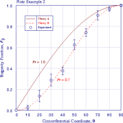
This example illustrates some of the additional capabilities of plotc. It draws the same two curves as in the first example, along with symbols representing experimental data with error bars. This time the MODEC = 20 option is used, and the coordinates of the curves are stored in a separate file. Text strings are drawn on the plot to label the two curves, a legend is added, and color is used.
The namelist input file is listed below, along with explanatory notes for each line. Remember that with namelist input each line starts in column 2 or higher.
 &ptype
  ncurv=-2, nsymb=1,                    Plot two curves and one set of symbols.
  rgbcrv(1,1)=0.5,0.0,0.0,              Colors "maroon" and red for curves.
  rgbcrv(1,2)=1.0,0.0,0.0,
  rgbsym(1,1)=0.0,0.0,0.5,              Use dark blue for symbols.
  ititle=1,1,1,                         Include plot and axis titles.
  fonts='H','R','R','R',                Use Helvetica for labels, Times-Roman otherwise.
  ilegnd=1,                             Add a legend.
     xleg=7.5, yleg=.9,                 Legend position.
     aleg(1,2)='Theory A',              Legend contents, column 2.
               'Theory B',
               'Experiment',
     ilegbx=1,                          Draw a box around legend.
     ilclr=1,                           Use curve/symbol colors for text.
  astr='\ftIPr \ftR = 1.0',             Add these text strings to plot.
       '\ftIPr \ftR = 0.7',
     xstr=25.,35., ystr=.45,.28,        Locations for strings.
     isizes=16,16,                      Point sizes for strings.
     salign(1)='RIGHT',                 Right-align first string.
     rgbstr(1,1)=0.5,0.0,0.0,           Colors "maroon" and red for strings.
     rgbstr(1,2)=1.0,0.0,0.0,
  modec=20,                             Get curve coordinates from a table.
     ifilec=1, irewc=1,                 Separate file for table, rewind between curves.
  modep=4,                              Get symbol sets as x, then y, free-form.
  iebar=1,                              Add centered error bars, length is fraction of y value.
 &end
 &axes
  iscale=1,                             Specify scales for both axes.
  xmin=0., xmax=90., xlen=6., nintx=9,  x-axis information.
  ymin=0., ymax=1.,  ylen=6., ninty=5,  y-axis information.
  ixaxis=2, iyaxis=2,                   Draw grid lines.
  rgbax=0.0,0.0,0.5,                    Dark blue for axes.
 &end
Circumferential Coordinate, \561        x-axis title.
Bogosity Function, \ftIF\sub[\542]      y-axis title.
Plotc Example 2                         Plot title.
51                                      Number of points, curve 1.
1 2                                     Use col. 1 for x, col. 2 for y.
51                                      Number of points, curve 2.
1 3                                     Use col. 1 for x, col. 3 for y.
10                                      Symbol set 1 x and y coordinates, error bar data.
0. 10. 20. 30. 40. 50. 60. 70. 80. 90.
0.00000 0.02447 0.13552 0.28711 0.37566 0.62434 0.74088 0.90451 0.96489 1.00000
0.      0.9     0.4     0.2     0.1     0.075   0.05    0.05    0.02    0.01
The table defining the curve coordinates is stored in a separate file, listed below.
 0.0   0.00000   0.00000
 1.8   0.03141   0.00099
 3.6   0.06279   0.00394
 5.4   0.09411   0.00886
 7.2   0.12533   0.01571
 9.0   0.15643   0.02447
10.8   0.18738   0.03511
12.6   0.21814   0.04759
14.4   0.24869   0.06185
16.2   0.27899   0.07784
18.0   0.30902   0.09549
19.8   0.33874   0.11474
21.6   0.36812   0.13552
23.4   0.39715   0.15773
25.2   0.42578   0.18129
27.0   0.45399   0.20611
28.8   0.48175   0.23209
30.6   0.50904   0.25912
32.4   0.53583   0.28711
34.2   0.56208   0.31594
36.0   0.58779   0.34549
37.8   0.61291   0.37566
39.6   0.63742   0.40631
41.4   0.66131   0.43733
43.2   0.68455   0.46860
45.0   0.70711   0.50000
46.8   0.72897   0.53140
48.6   0.75011   0.56267
50.4   0.77051   0.59369
52.2   0.79015   0.62434
54.0   0.80902   0.65451
55.8   0.82708   0.68406
57.6   0.84433   0.71289
59.4   0.86074   0.74088
61.2   0.87631   0.76791
63.0   0.89101   0.79389
64.8   0.90483   0.81871
66.6   0.91775   0.84227
68.4   0.92978   0.86448
70.2   0.94088   0.88526
72.0   0.95106   0.90451
73.8   0.96029   0.92216
75.6   0.96858   0.93815
77.4   0.97592   0.95241
79.2   0.98229   0.96489
81.0   0.98769   0.97553
82.8   0.99211   0.98429
84.6   0.99556   0.99114
86.4   0.99803   0.99606
88.2   0.99951   0.99901
90.0   1.00000   1.00000
The following terminal session shows how you would use the above input files to create your plot. Lines in slanted type are entered by the user. The remainder are printed by the computer. This example assumes the plotc namelist input file is bogus2.plotin, and that the file containing the coordinates of the curves is bogus2.coords.
plotc -a bogus2.coords bogus2.plotin
Using namelist input file bogus2.plotin
Using unit 8 input file bogus2.coords

PostScript output is in plotc.ps
As in the previous example, the OpenGL plot will appear in a window
on the screen, and the PostScript plot will be written into the file
plotc.ps.
The PostScript plot is shown below.
Suppose, for some strange reason, you wanted a plot of a square inscribed in a circle. You could create a file named coors.f90, containing the following COORS routine to be used with plotc. It computes coordinates for two curves. The first is the circle, centered at (0,0) with a radius of 1. The second curve is the inscribed square.
      subroutine coors (x,y,np,icurv,xtitle,ytitle,ptitle)
!
!          This subroutine is used as an example to illustrate the use
!     of the plotting program Plotc.  It returns x-y coordinates for a
!     plot of a square inscribed in a circle (not real useful, but this
!     is only an introductory example, after all.)
!
      dimension x(1),y(1)
      character*(*) xtitle,ytitle,ptitle
      save radius
      data pi /3.1415927/

!
!-----First curve, the circle
!
      if (icurv == 1) then
!--------Set number of points in curve
         np = 101
!--------Define x-y coordinates for circle
         radius = 1.
         dtheta = (2.*pi)/float(np-1)
         do i = 1,np
            theta = dtheta*float(i-1)
            x(i) = radius*cos(theta)
            y(i) = radius*sin(theta)
         end do

!
!-----Second curve, the inscribed square
!
      else if (icurv == 2) then
!--------Half-length of side
         side2 = sqrt(radius/2.)
!--------x-y coordinates of square corners
         x(1) = -side2
         y(1) =  side2
         x(2) =  side2
         y(2) =  side2
         x(3) =  side2
         y(3) = -side2
         x(4) = -side2
         y(4) = -side2
         x(5) = x(1)
         y(5) = y(1)
!--------Total number of points in curve
         np = 5
      endif

      return
      end
The above user-written file coors.f90 must then be compiled and linked into the executable during the build process, as described in the section Installing Plotc.
You'll also need a namelist file for the plotc input. Remember that with namelist input each line starts in column 2 or higher. The input file might look like:
 &ptype
  ncurv=2,                              Plot two curves (circle and square).
 &end
 &axes
  iscale=1,                             Specify scales for both axes.
  xmin=-1., xmax=1., ymin=-1., ymax=1., Axes starting and ending values.
  xlen=6., ylen=6.,                     Axes lengths.
  ixaxis=3, iyaxis=3,                   Suppress plotting of both axes.
 &end
Note that even though we are suppressing the plotting of both axes, values for XMIN, XMAX, XLEN, etc., must still be specified to allow plotc to transform user's units into relative units.
The following terminal session shows how you would then create your plot. Lines in slanted type are entered by the user. The remainder are printed by the computer. This example assumes that the plotc namelist input file is cirsq.plotin.
plotc cirsq.plotin
Using namelist input file cirsq.plotin

PostScript output is in plotc.ps
As in the previous example, the OpenGL plot will appear in a window
on the screen, and the PostScript plot will be written into the file
plotc.ps.
The PostScript plot is shown below.

Last updated 2 Nov 2005