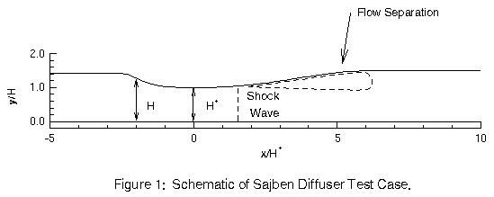
Figure 1. Flow field for Sajben transonic diffuser
Figure 1. Flow field for Sajben transonic diffuser
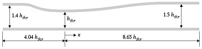
Figure 2. Geometry for the Sajben transonic diffuser,
where hthr is 1.7322 inches
This validation study examines transonic air flow through a converging-diverging diffuser with a normal shock wave present. Both the structured and unstructured flow solvers were used, as well as the SA and SST turbulence models. The results were compared with experimental data.
All of the archive files of this validation case are available in a Unix tar file: sajben.tar. The files can then be accessed by the commands:
tar -xvof sajben.tar
Four grids were used to simulate the diffuser cases. The Gridgen grid generation package was used to create these grids. The first grid (sajben_s_2d.cgd) is a structured 2-dimensional grid with 81 axial points and 51 vertical points. The y+ value one point from the wall was approximately equal to 1.0. This grid is shown in Figure 3.
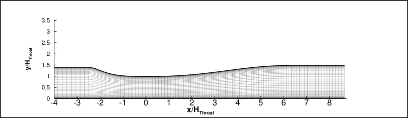
Figure 3. 2-Dimensional Structured Grid.(H throat is 1.7322 inches.)
The second grid (sajben_s_3d.cgd) was 3-dimensional with hexagonal cells. To construct it, the 2-dimensional structured grid was extruded 2-cells in the z-direction. The depth of the grid was 1 inch. This grid is could be used as a structured grid with the structured solver, however for this study, it was saved in "unstructured" format and used with the WindUS unstructured flow solver.
The third grid (sajben_u.cgd) was unstructured and 3-dimensional. The perimeter of the diffuser has a structured (hexahedral) grid cells and the center of the diffuser has unstructured (tetrahedral) cells. This grid has 36,714 grid points with 201 points in the axial direction and 2 points in the z-direction. The depth of the grid in the z-direction is 1 inch. This grid is shown in Figure 4.
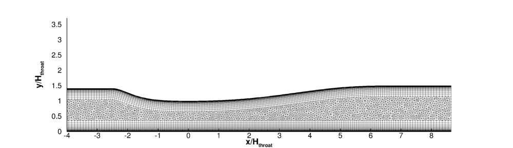
Figure 4. 3-Dimensional diffuser grid with structured (hexahedral) grid around the edge of the diffuser and unstructured (tetrahedral) grid through the center.
In the last grid (grid_u_ext.cgd), a constant area duct section was added to the unstructured grid. It was 10 throat-heights long and had 101 axial points. The extension was added to avoid separation at the outflow boundary plane, as will be discussed below. The duct grid with a portion of the constant-area extension is shown in Figure 5.
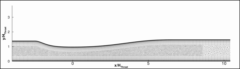
Figure 5. 3-Dimensional diffuser grid show part of the constant area extension.
After the cgd file was exported from Gridgen, CFPART was used to add lines to the grid in preparation to be solved with Wind-US Gauss-Seidel implicit solver. In Table 1, both the Common and Gridgen versions of the grid are attached as well as the CFPART script used to add lines.
| Gridgen (*.gg) | Common Grid (*.cgd) | Pre-Processing (*.inp) |
|---|---|---|
| sajben_s_2d.gg | sajben_s_2d.cgd | Not Applicable |
| sajben_s_3d.gg | sajben_s_3d.cgd | cfpart_s_3d.inp |
| sajben_u.gg | sajben_u.cgd | cfpart_u.inp |
| sajben_u_ext.gg | sajben_u_ext.cgd | cfpart_u_ext.inp |
| Pressure (psia) | Temperature (R) | Mach Number | |
| Freestream | 19.58 | 540 | 0.9 |
Boundary conditions were selected to generate the Strong Shock case described in Study #2 . The upper and lower boundaries were viscous walls. The Reflection/Symmetry BC was imposed on the two sidewalls (parallel to the page). On the inflow boundary (on the left in the images), FREESTREAM conditions were imposed using a total pressure of 19.58 psi and total temperature of 540 R. For the cases run using the standard length grids, sajben_s_2d.cgd, sajben_s_3d.cgd and sajben_u.cgd, the outflow boundary, x/HThroat=8.65, had an OUTFLOW BC with 14.1 psi static pressure imposed. For the case run using the grid with the downstream extension, sajben_u_ext.cgd, the downstream pressure at the duct exit, x/HThroat=18.65, was set to a higher value of 14.775 psi. This was required to obtain the correct pressure of 14.1 psi at x/HThroat=8.65. (Note that in the extension, the boundary layers continue to grow, causing the effective area to decrease, and the flow to accelerate. A higher pressure at the extension exit is required to maintain the desired mass flow and shock position in the diffuser.)
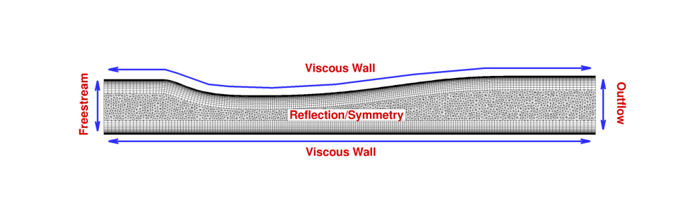
Figure 6. Boundary conditions.
The solution was considered converged when the centerline pressures were no longer changing and the residuals had dropped several orders of magnitude then leveled off.
The inputs for the seven cases are given in Table 3 below. The cases are named according to the grid (i.e. "s_2d", "s_3d", "u_" or "u_ext") and the turbulence model ("SA" or "SST") used. Note that in case u_SST, a smaller maximum CFL number, 50, and was required for convergence, compared to the value of 100 used with the SA model. This was not required for case u_ext_SST. Different versions of the code were used based on the most recent available at run time.
| Case | s_2d_SA | s_2d_SST | s_3d_SA | s_3d_SST | u_SA | u_SST | u_ext_SST |
|---|---|---|---|---|---|---|---|
| Version | Wind-US 3.139 | Wind-US 3.145 | Wind-US 3.139b | Wind-US 3.139b | Wind-US 3.146 | Wind-US 3.146 | Wind-US 3.139b |
| Solver | Structured | Structured | Unstructured | Unstructured | Unstructured | Unstructured | Unstructured |
| Grid | Structured | Structured | Structured | Structured | Unstructured | Unstructured | Unstructured |
| Cycles | 30000 | 30000 | 30000 | 30000 | 21000 | 21000 | 30000 |
| Converge Order | 10 | 10 | 10 | 10 | 10 | 10 | 10 |
| Method | Default | Default | IMPLICIT UGAUSS LINE EXACT_LHS VISCOUS_JACOBIAN FULL CONVERGE FREQUENCY 11 SUBITERATIONS 6 | IMPLICIT UGAUSS LINE EXACT_LHS VISCOUS_JACOBIAN FULL CONVERGE FREQUENCY 11 SUBITERATIONS 6 | IMPLICIT UGAUSS LINE EXACT_LHS VISCOUS_JACOBIAN FULL CONVERGE FREQUENCY 11 SUBITERATIONS 6 | IMPLICIT UGAUSS LINE EXACT_LHS VISCOUS_JACOBIAN FULL CONVERGE FREQUENCY 11 SUBITERATIONS 6 | IMPLICIT UGAUSS LINE EXACT_LHS VISCOUS_JACOBIAN FULL CONVERGE FREQUENCY 11 SUBITERATIONS 6 |
| CFL | 1.0 | 1.0 | AUTO DECREASE 2 CFLMIN 1 CFLMAX 100 | AUTO DECREASE 2 CFLMIN 1 CFLMAX 100 | AUTO DECREASE 2 CFLMIN 1 CFLMAX 100 | AUTO DECREASE 2 CFLMIN 1 CFLMAX 50 | AUTO DECREASE 2 CFLMIN 1 CFLMAX 100 |
| DQ Limiter | Default | Default | DQ LIMITER ON RELAX 0.5 | DQ LIMITER ON RELAX 0.5 | DQ LIMITER ON RELAX 0.5 | DQ LIMITER ON RELAX 0.5 | DQ LIMITER ON RELAX 0.5 |
| Mut Limiter | Default | Default | MUT LIMITER 50 | MUT LIMITER 50 | MUT LIMITER 50 | MUT LIMITER 50 | MUT LIMITER 50 |
| Dissipation | Default | Default | Default | Default | TVD VENKAT 3.0 KVENKAT 0 | TVD VENKAT 3.0 KVENKAT 0 | Default |
| Boundaries | Default | Default | IMPLICIT BOUNDARY ON | IMPLICIT BOUNDARY ON | IMPLICIT BOUNDARY ON | IMPLICIT BOUNDARY ON | IMPLICIT BOUNDARY ON |
| RHS | HLLE SECOND | HLLE SECOND | HLLE SECOND | HLLE SECOND | HLLE SECOND | HLLE SECOND | HLLE SECOND |
| Solver Stages | First Order for First 1000 iter, then Switch to Second Order | First Order for First 1000 iter, then Switch to Second Order | First Order for First 500 ter, then Switch to Second Order | First Order for First 500, then Switch to Second Order | First Order for First 1000 iter, then Switch to Second Order | First Order for First 1000 iter, then Switch to Second Order | First Order for First 500 iter, then Switch to Second Order |
| Turbulence | SPALART | SST | SPALART | SST | SPALART | SST | SST |
The input data file and output list and solution files are given in Table 4.
| Case | Input File | Grid File | List File | Solution File |
|---|---|---|---|---|
| s_2d_SA | s_2d_sa.dat | sajben_s_2d.cgd | s_2d_sa.lis | s_2d_sa.cfl |
| s_2d_SST | s_2d_sst.dat | sajben_s_2d.cgd | s_2d_sst.lis | s_2d_sst.cfl |
| s_3d_SA | s_3d_sa.dat | sajben_s_3d.cgd | s_3d_sa.lis | s_3d_sa.cfl |
| s_3d_SST | s_3d_sst.dat | sajben_s_3d.cgd | s_3d_sst.lis | s_3d_sst.cfl |
| u_SA | u_sa.dat | sajben_u.cgd | u_sa.lis | u_sa.cfl |
| u_SST | u_SST.dat | sajben_u.cgd | u_SST.lis | u_SST.cfl |
| u_ext_SST | u_ext_SST.dat | sajben_u_ext.cgd | u_ext_SST.lis | u_ext_SST.cfl |
Each case has a post-processing script that calculates centerline pressures along the inside top and bottom walls of the diffuser. A "results" folder must be created in the scripts' directory in order to create the output files. The cgd and cfl files can be loaded into Tecplot using the Common File Format Loader. Variables can then be measured using the "Probe" tool. "Analyze>Calculate" can be used to calculate more variables and "Data>Alter" can be used to rescale data.
| Case | Script |
|---|---|
| s_2d_SA | s_2d_sa.postproc |
| s_2d_SST | s_2d_sst.postproc |
| s_3d_SA | s_3d_sa.postproc |
| s_3d_SST | s_3d_sst.postproc |
| u_SA | u_sa.postproc |
| u_SST | u_SST.postproc |
| u_ext_SST | u_ext_SST.postproc |
Mach contours are shown for the cases run using the ustructured solver on the unstructured grids in Figures 7 - 9. A normal shock wave is seen just downstream of the throat, and the flow separates on the top wall. In the experiment, the flow reattached near x/H throat= 6.4. For the cases run on the structured grids, the solutions show reattachment a little downstream of the experimental location, at about x/HThroat=7.5. For the cases run on the unstructured grid, sajben_u.cgd, the flow did not reattach and is separated at the outflow plane. (See case u_SA in Figure 7 and case u_SST in Figure 8.) This prompted the use of grid sajben_u_ext.cgd, as shown by case u_ext_SST in Figure 9. The flow is attached at the new outflow plane, and allowing the flow in the original duct to reattach near x/HThroat=7.4 which is similar to the solutions run using the structured grids.
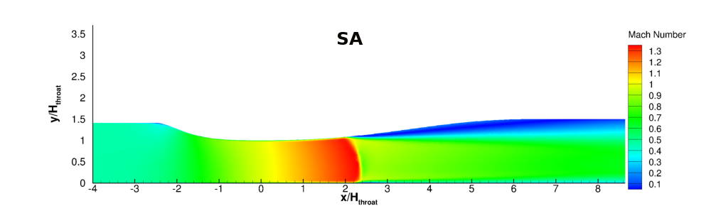
Figure 7. Mach contours for case u_SA.
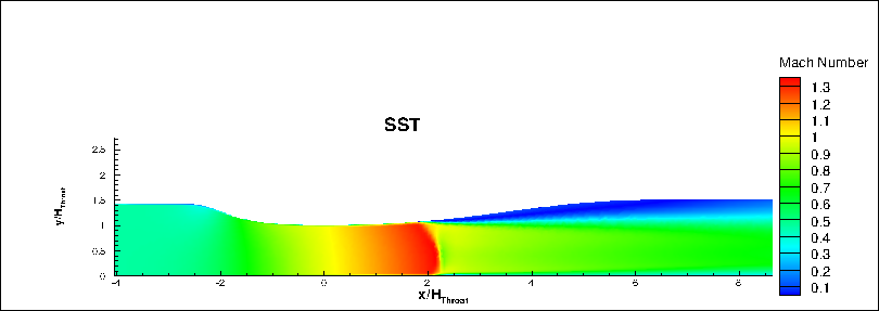
Figure 8. Mach contours for case u_SST.
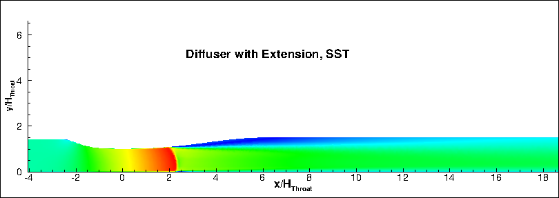
Figure 9. Mach contours for case u_ext_SST.
The static pressure distributions on the top and bottom wall are given in Figures 10 and 11 for simulations using the SA turbulence model and Figures 12 and 13 for simulations using the SST turbulence model. The results indicate generally good agreement with experimental data. For the SA and SST simulations using the unstructured solver, u_SA, and u_SST, respectively, there is separated flow at the outflow boundary. Adding the constant-area grid extension allowed the flow to reattach before reaching the outflow boundary. This improved the shock position slightly, as shown in Figures 12 and 13 by the u_ext_SST curve.
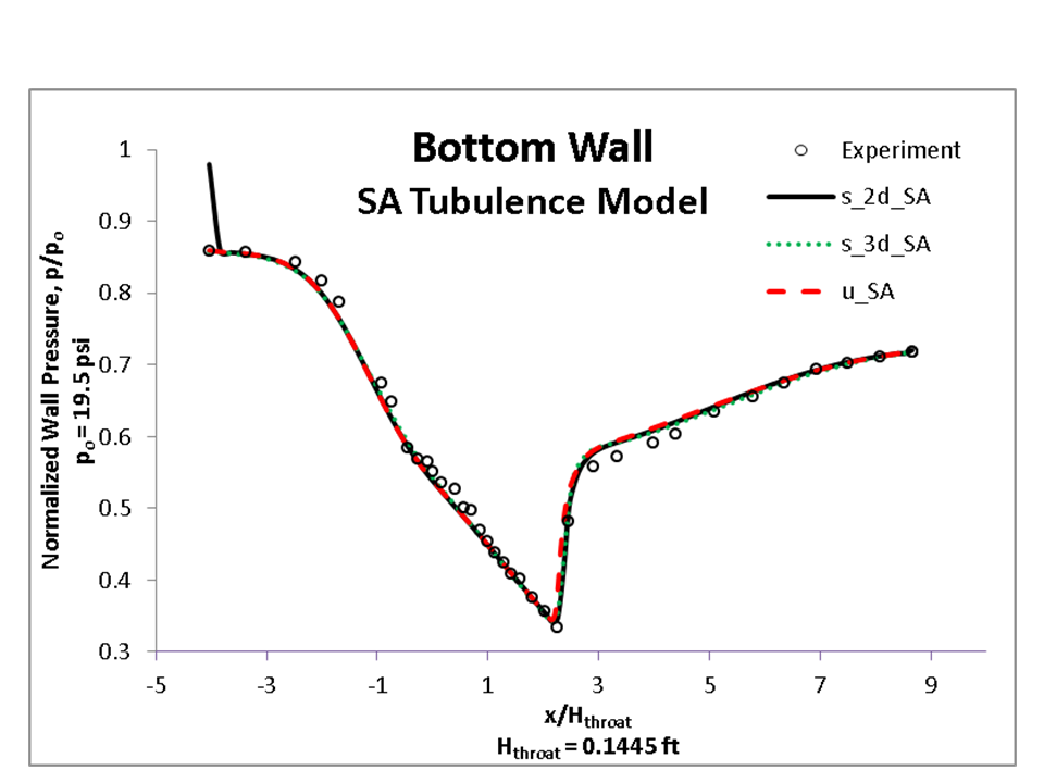
Figure 10. Bottom wall centerline pressures for simulations using the SA model
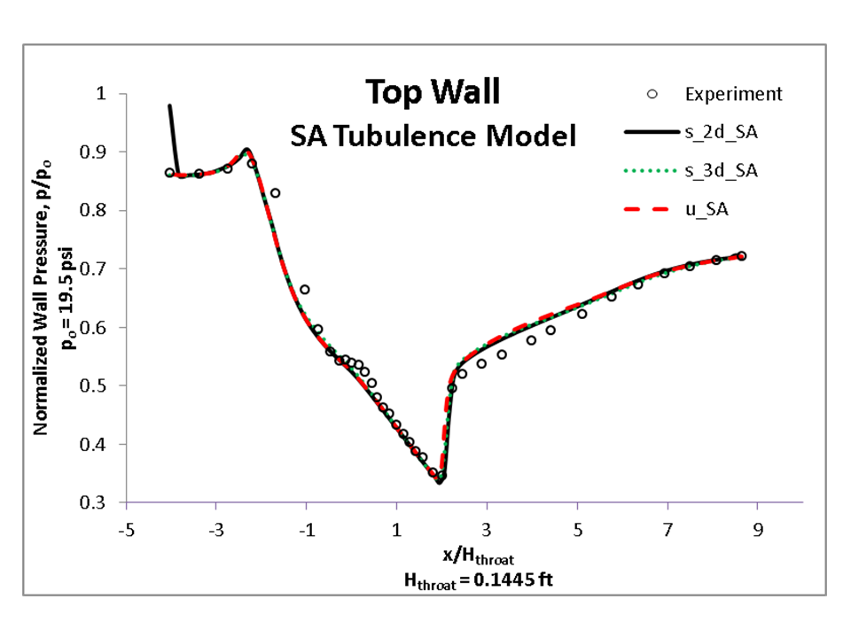
Figure 11. Top wall centerline pressures for simulations using the SA model
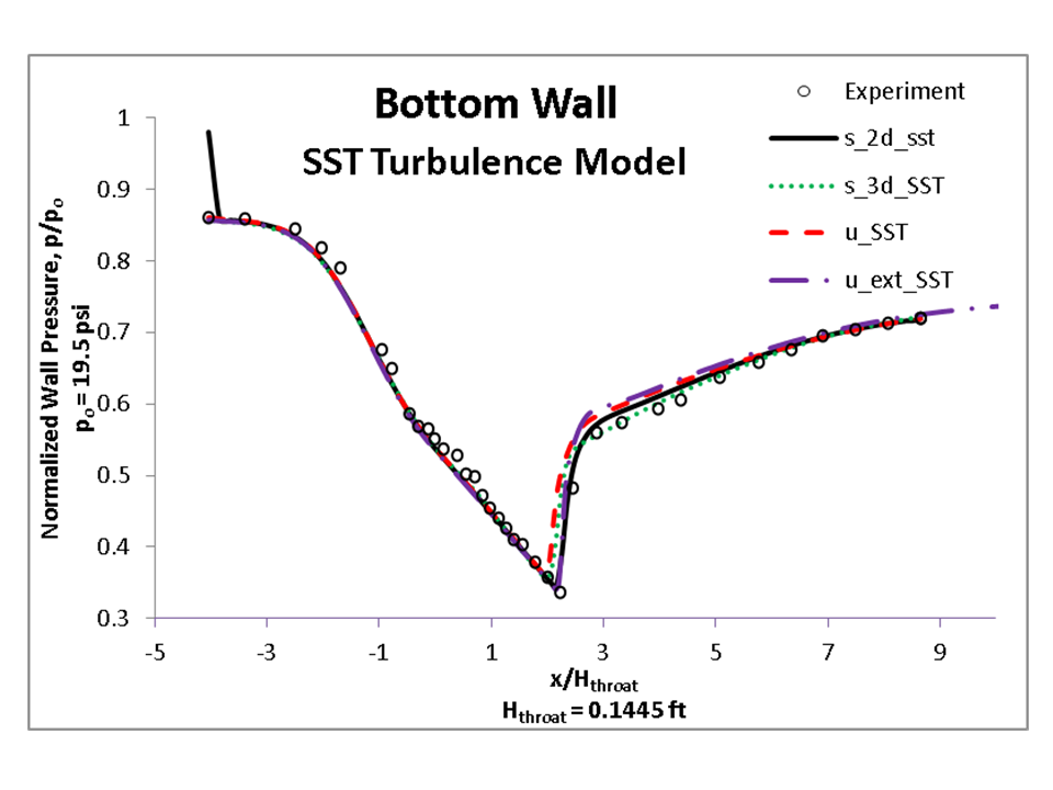
Figure 12. Bottom wall centerline pressures for simulations using the SST model
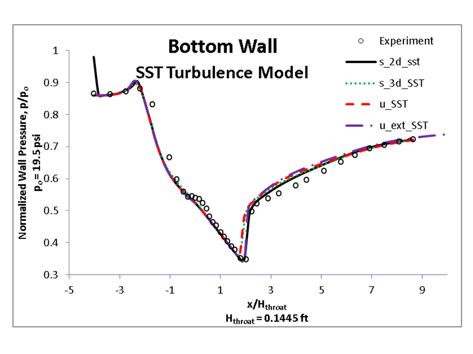
Figure 13. Top wall centerline pressures for simulations using the SST model
The velocity profiles are shown in Figure 14 for cases u_SA, u_SST and u_ext_SST. Prediction of separation and reattachment is a significant challenge in CFD, and in general, not accurately predicted. Adding the constant area extension to the duct is an important step to improving the prediction of reattachment. As seen below, only case u_ext_SST, which has the duct extension, has predicted the reattachment of the flow as shown at x/H = 7.5. Both cases u_SA and u_SST have separated flow at the outflow boundary plane, impacting the solver's ability to allow the flow to reattach.
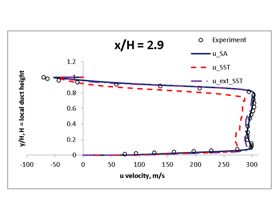
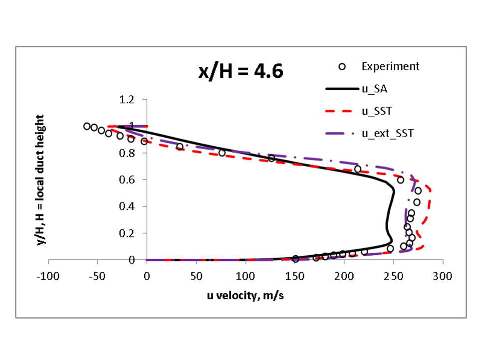
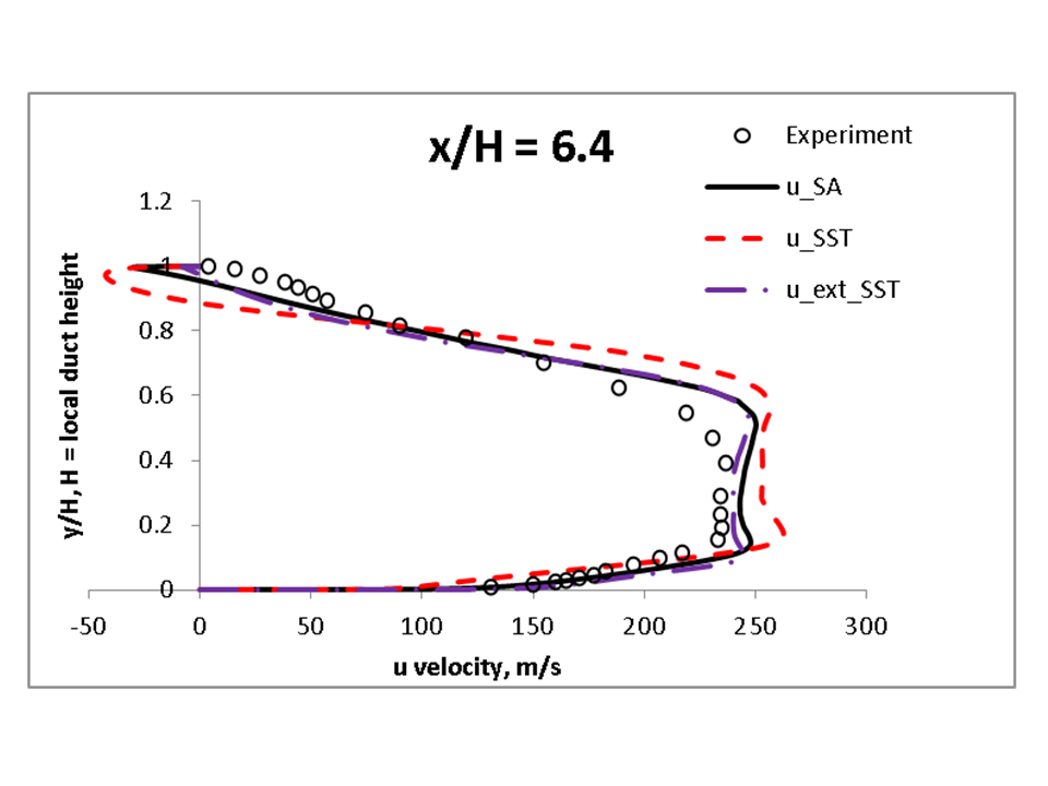
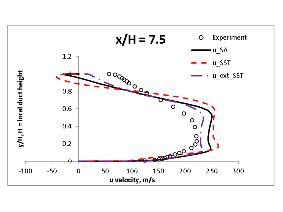
Figure 14. Velocity Profiles
This validation test case was performed by Julianne Dudek. Contact: Julianne Dudek, (216) 433-2188. MS 5-12, NASA Glenn Research Center, 21000 Brook Park Road, Cleveland, Ohio, 44135.