Figure 1. Shock tube at initial state.
Figure 1. Shock tube at initial state.
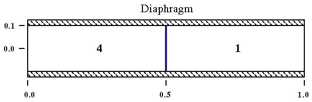
This validation case involves an unsteady flow in a shock tube. The tube is a cylinder. A diaphragm separates the gas at two states. Fig. 1 shows the shock tube at the initial states.
| Region | Pressure (psia) | Temperature (R) | Density |
|---|---|---|---|
| 1 | 1.0 | 416.0 | 0.125 |
| 4 | 10.0 | 520.0 | 1.0 |
As the diaphragm bursts a shock, slip surface, and expansion waves form a propagate through the tube. Fig. 2 shows the state of the flow a short time after the burst of the diaphragm.
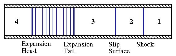
Figure 2. Shock tube shortly after diaphragm has burst.
The shock tube is a cylinder of length 1.0 ft and a inside radius of 0.1 ft. Fig. 1 shows the geometry.
The tube is closed at the ends, thus all boundaries of the computational domain are ideally solid walls. The inside surface of the tube is assumed a slip surface. Since the time span of the unsteady flow is short, the waves never reach the end walls, and so, conditions at these boundaries are held fixed.
The classical shock tube solution provides data for comparison. The text by Anderson discusses this solution. The Fortran program stubex.f creates the data files containing the pressure stp.dx, density str.dx, axial velocity stu.dx, and Mach number stm.dx along the tube at the final time, which is at t = 2.11725E-04 seconds. The pressure and density has been non-dimensionalized by the pressure at state 4.
The computational grid was generated by the Fortran program stubeic.f. The number of axial and radial grid points are input and then are evenly spaced. Fig. 3 below shows an example planar grid.
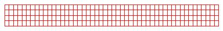
Figure 3. Computational grid (coarsened for display).
| Study | Category | Person | Comments |
|---|---|---|---|
| Study #1 | Example | J.W. Slater | Explicit, Runge-Kutta Operator. |
| Study #2 | Example | J.W. Slater | Explicit. Comparison with NPARC. |
| Study #3 | Example | J.C. Dudek | Implicit, Point Jacobi Operator. |
1. Anderson, J.D., Modern Compressible Flow , McGraw Hill Inc., New York, 1984.