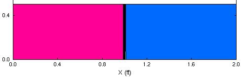
Figure 1. Mach number contours for inviscid Mach 1.3 flow through a normal shock.
Figure 1. Mach number contours for inviscid Mach 1.3 flow
through a normal shock.
This verification case involves the steady, inviscid, adiabatic Mach 1.3 flow with a normal shock. Supersonic flow enters the normal shock and subsonic flow exits the shock. This flow is a classic, fundamental supersonic flow whose analytic solution is exact and can be found in any compressible flow textbook, such as the book by Anderson.
The supersonic conditions are presented in Table 1 and represent the reference conditions. The choice of pressure and temperature are arbitrary and do not change the basic character of the flow for perfect gases.
| Mach | Pressure (psia) | Temperature (R) | Angle-of-Attack (deg) | Angle-of-Sideslip (deg) |
|---|---|---|---|---|
| 1.3 | 10.0 | 520.0 | 0.0 | 0.0 |
The geometry is a straight duct of length 2.0 ft with a diameter of 1.0 ft.
An analytic solution for the inviscid, supersonic, steady, adiabatic flow through a normal shock is well known and presented in any compressible flow text book. Table 3 presents the solution for a Mach 1.3 supersonic flow. The subscript 1 refers to the supersonic side of the shock, while the subscript 2 refers to the subsonic side of the shock.
Since the flow is supersonic, the inflow boundary I1 of the domain is specified as FROZEN. The outflow boundary IMAX is specified as an OUTFLOW boundary where the Mach number is specified. The J1 boundary is a singular axis and is specified as an INVISCID WALL. The JMAX boundary is the casing of the duct and is specified as an INVISCID WALL. The K1 and KMAX boundaries are specified as REFLECTION planes.
The grid is generated using the Fortran 90 program normic.f90 with a grid size of (202x11x5). The grid is uniformly spaced in all directions. The grid file is norm.x and is in Plot3d format (unformatted, multi-zone, 3D, whole, single-precision). A formatted Plot3d file (formatted, multi-zone, 3D, whole, double-precision) is available as norm.x.fmt. This is converted to the common grid file format as norm.cgd.
The boundary conditions are implemented through GMAN as
gman < gman.com
The initial flow conditions are created through the Fortran program normic.f90 to correspond to the analytic solution for the normal shock. The shock is placed at x = 1.0 ft and the even number of grid points assures that the shock is initially placed between two grid points.
The computation was performed using the time-marching capabilities of Wind-US 3.0 to march to a steady-state (time asymptotic) solution. Local time stepping is used at each iteration. The time-marching is performed until convergence criteria is achieved.
The input data file for the WIND computation is norm.dat. Much of the default settings are used. The CFL number was 1.5 and the computation was run for 1000 iterations.
The input and output files for the Wind-US computation are listed in Table 2.
| File | Wind-US 3.139 |
|---|---|
| Grid | norm.cgd |
| Input Data File | norm.dat |
| Solution | norm.cfl |
| List / Residual | norm.lis |
The residual information was read from the WIND list files using the RESPLT utility and plotted using CFPOST,
resplt < resplt.nsl2.com
cfpost < cfpost.nsl2.com
The CFPOST utility was used to obtain information from the solution.
Flowfield Mach Number Contours. The Mach number contours for the flow field can be generated by
cfpost < cfpost.mach.com
Properties at J1. The properties along J1, which is the axial direction, are output to the GENPLOT file J1.gen by
cfpost < cfpost.J1.com
The average properties aft of the shock are computed using the Fortran program avg.f. It simply sums up the values after x of 1.2 and averages them. These values are expected be constant.
avg < J1.wind.gen
avg < J1.wind.gen
avg < J1.nparc.gen
A comparison with theoretical values of the properties behind the shock are provided below. Results from Wind-US are listed along with results from an earlier version of WIND and NPARC. All computations provide excellent agreement with the theoretical values.
| Computation | Exact | Wind-US 3.139 | WIND 2.172 | NPARC 3.0 |
|---|---|---|---|---|
| M2 | 0.7860 | 0.7860 | 0.7860 | 0.7860 |
| p2 / p1 | 1.8050 | 1.8050 | 1.8049 | 1.8049 |
| pt2 / pt1 | 0.9794 | 0.9794 | 0.9794 | 0.9794 |
| rho2 / rho1 | 1.5157 | 1.5159 | 1.5156 | 1.5156 |
| T2 / T1 | 1.1909 | 1.1907 | 1.1909 | 1.1908 |
| Tt2 / Tt1 | 1.0000 | 1.0000 | 1.0000 | 1.0000 |
Anderson, J.D., Modern Compressible Flow , McGraw Hill Inc., New York, 1984.
Questions or comments about this case can be sent be emailed to John W. Slater,
NASA John H. Glenn Research Center, MS 5-12
21000 Brookpark Road
Cleveland, Ohio 44135
Phone: (216) 433-8513
e-mail: John.W.Slater@nasa.gov