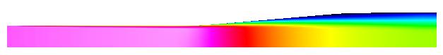
Figure 1. The shading of the Mach number for the Fraser subsonic conical diffuser.
Figure 1. The shading of the Mach number for the Fraser
subsonic conical diffuser.
This test case computes incompressible turbulent flow in a conical diffuser, and is referred to as the Fraser (flow A) case from the 1968 AFOSR-IFP Stanford Conference on Computation of Turbulent Boundary Layers. The geometry consists of a straight section of pipe followed by a 5 degree half-angle conical diffuser. The core Mach number at the diffuser entrance is 0.15 (52 m/s), and the Reynolds number based on pipe diameter is approximately 500,000. (This is an NPARC model validation case, which can be found at the NPARC Validation Web page.)
This document is the HTML version of the README file created by Julianne Dudek.
The geometry consists of a straight section of pipe followed by a 5 degree half-angle conical diffuser.
The boundary conditions, which were set using GMAN are:
(1) I1 - inflow
(2) IMAX - confined outflow
(3) J1 - inviscid wall
(4) JMAX - viscous wall
The units were set to feet. The resulting grid and boundary condition file is subsdif.cgd . The script file containing the above GMAN inputs is called gman.jou .
The grid used is structured and has 121 axial points and 71 radial points. It is packed at the wall such that y+=1 at the first point from the wall. It is also packed axially at the inflow boundary to resolve large axial flow gradients.
The grid was obtained from the NPARC validation archive (http://info.arnold.af.mil/nparc/model/subsdif/case01/plotx1.bin). The CFCNVT utility was used to convert plotx1.bin, which was in PLOT3D format (2D/multigrid/formatted), to a .cgd file (subsdif.cgd) which could be read by GMAN and WIND. The grid is also available as a 2D, single-zone, formatted Plot3d file as subsdif.x.fmt .
| Topology: | Structured, multi-block |
| Number of Blocks: | 1 |
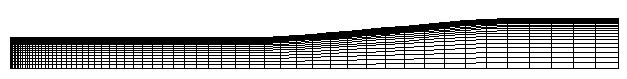
Figure 2. A plot of the grid for the subsonic diffuser.
The table below lists the names of the common grid files (*.cgd) and the Plot3d grid file for the grid. The Plot3d files are two-dimensional, whole, single-block and Iris binary. Picking the file name will allow you to download the file to your local directory.
| Grid | Density | CGD File | Plot3d Grid File |
|---|---|---|---|
| A | 121 x 71 | subsdif.cgd | subsdif.x.bin |
The steady-state flow was computed for the grid. Table 2 lists the name of the input data file for the run (picking the file name will cause the ASCII file to be displayed). The run used the default input values for WIND. A CFL number of 1.3 was used. The computations were performed for a set number of iterations until that the convergence histories leveled out.
| Grid | Input Data File | CFL Number | Iterations | CPU Time (sec) |
|---|---|---|---|---|
| A | subsdif.dat | 1.3 | 60000 | - |
| Grid | List File | L2 Residual | CFL File | Mass Flux | Plot3d Solution |
|---|---|---|---|---|---|
| A | subsdif.lis | subsdif.resl2 | subsdif.cfl | subsdif.mflux | subsdif.q.bin |
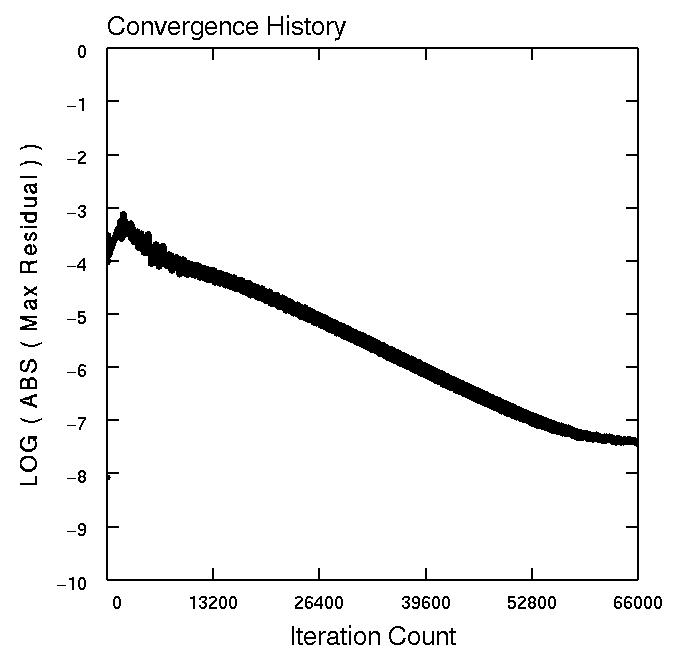
Figure 2. The plot of the convergence history for the
WIND computations of flow in the subsonic diffuser.
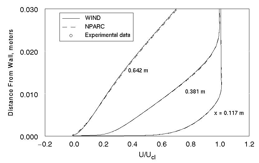
Figure 3. The plot of the velocity distributions
along the surface of the subsonic diffuser.
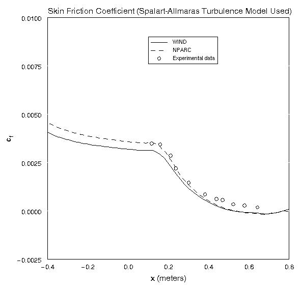
Figure 4. The plot of the skin friction coefficient
along the surface of the subsonic diffuser.
Fraser, H.R., "The Turbulent Boundary Layer in a Conical Diffuser," Journal of the Hydraulic Division , Proceedings of the American Society of Civil Engineers, pp. 1684-1-17, June 1958.
Dudek, J.C., N.J. Georgiadis, and D.A. Yoder, "Calculation of Turbulent Subsonic Diffuser Flows Using the NPARC Navier-Stokes Code," AIAA Paper 96-0497, January 1996.