 NPARC Alliance V&V Archive
This validation study examines the separated flow through a 2D asymmetric diffuser using the Menter SST, Chien k-e, and Spalart-Allmaras turbulence models. It was completed in order to investigate WIND's ability to predict the correct separation behaviors with smooth walls and adverse pressure gradients. The inlet flow is two-dimensional, incompressible, turbulent, and fully-developed channel flow with a Reynolds number of 20,000 based on the centerline velocity and the channel height. The prediction of the separation and reattachment points and the extent of the recirculation in these types of problems is particularly challenging for computational models. This flow has been experimentally studied at least by two different research groups: Obi et al at Keio University in Japan, and Buice & Eaton at Stanford University. In this study, numerical results are compared with experimental data in the form of axial velocity plots and skin friction data.
Please Note: This webpage has been optimized to be viewed with Microsoft Internet Explorer.
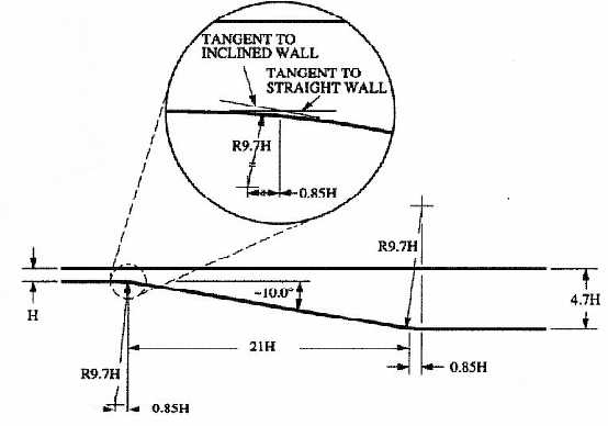
Figure 1. The geometrical description of the diffuser from Buice and Eaton.
The runtime files for the SST model case are contained in the Unix compressed tar file buice.tar.gz. The files can then be extracted by the unix command
uncompress -c buice.tar.gz | tar xvof -
The files buice.x, buice.cgd, buice.cfl and buice.dat are the grid file in plot3d format, grid file in WIND common file format, WIND solution file, and WIND input file, respectively. The original experimental data points can be found here.
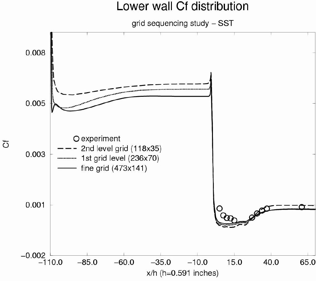
The 2D grid is contained in a PLOT3D grid file (unformatted, single-zone, whole, three-dimensional) named buice.x. It consists a single zone with grid dimensions 473 x 141 (Figure 2 left). The x- and y-axes are taken in the streamwise and straight-wall normal directions, respectively. The origin of the x-axis is located at the intersection of the tangents to the straight and inclined wall, as shown in Figure 1. The y-axis originates from the bottom wall of the downstream channel. The I1 surface is the inflow. The IMAX surface is the outflow. The J1 surface is the diffuser. The JMAX surface is the upper viscous wall. The common grid file is buice.cgd. Walls were clustered such that average y+ values were 1. The height H of the inflow domain is 0.591 inches. The grid was created with Pointwise, Inc's GRIDGEN software. The inflow region is 110H long. The lower wall of the diffuser section is at y = 0, and the section is 4.7H high and extends 56H downstream (of the ramp). Grid sequencing was used at 2 levels (118x35) and 1 level (236x70) to get an initial solution. Solutions obtained on a 1st level grid sequencing were very similar to solutions obtained on the full grid. All solutions presented here are with the full, unsequenced grid. A comparison of skin friction along the lower wall for the three grid levels using the SST model can be seen in Figure 2 (right). From this, it can be seen that the fine grid is sufficient to capture the flow effects especially in the diffuser region (x/H > 0).
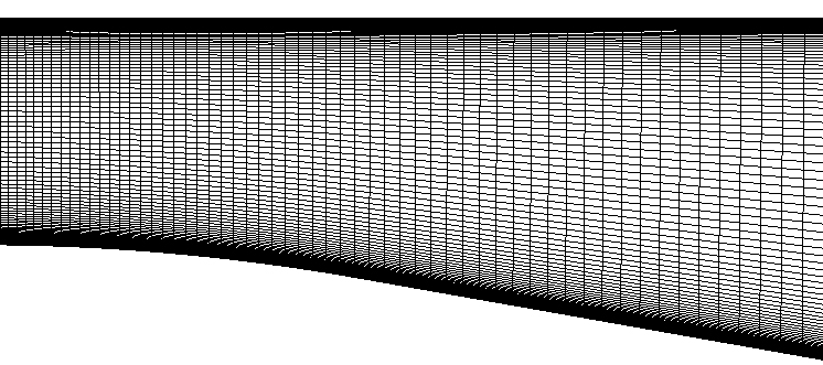
Figure 2. Zoomed view of computationl grid (left) and grid sequencing study for three grid levels (right).
The initial flow conditions are simply the conditions of the freestream keyword as presented in Table 1.
Table 1. Static Freestream conditions.
|
Mach |
Pressure (psia) |
Temperature (R) |
Angle-of-Attack (deg) |
Angle-of-Sideslip (deg) |
|---|---|---|---|---|
|
0.06 |
14.7 |
530.0 |
0.0 |
0.0 |
The bulk flow velocity Ub in the channel is 65 ft/sec, and the upstream channel centerline velocity is 1.14 Ub (=74.1 ft/sec). The static pressure was specified at the outflow BC (back pressure), and was adjusted slightly in order to obtain the correct Ub just upstream of the diffuser. The final pressure value for the SST model was 14.669 psi. This back pressure value was modified during the run cycle in order to obtain the same bulk flow velocity as the experiment just upstream of the diffuser. Another run was performed to investigate WIND's massflow specification option, and in order to conserve mass, WIND calculated and used a pressure of 14.6801 psi at the exit plane. About a 0.042 psi increase in back pressure was required for the SST model (compared with the S-A model). Assuming a static inflow temperature and pressure for normal wind tunnel conditions, and using the given Reynolds number of 20,000 and channel height H, the inlet Mach number (or flow velocity) of 0.06 was extrapolated and used to initialize the solution. From this, the bulk velocity just upstream of the diffuser was fine-tuned to match experimental conditions by slightly adjusting the back pressure (exit static pressure) while keeping the inflow static temperature and pressure specified in Table 1. The inflow conditions set with the arbitrary inflow keyword were the same as the reference conditions set with the freestream keyword.
The I1 inflow boundary is specified with a ARBITRARY INFLOW boundary condition (BC). Static values with “hold totals” were specified uniformily across the inflow plane. The IMAX boundary is specified with an OUTFLOW boundary condition. The J1 and JMAX boundaries are specified with an VISCOUS WALL boundary condition. These are set in GRIDGEN. This problem was initially tried with a freestream BC specifying both total and static values (using hold totals) which presented unacceptable results and sluggish convergence. Profiles upstream of the diffuser were correct but axial velocity profiles in the diffuser itself were not matching experimental data (although, qualitatively, the solution looked correct). Using the arbitrary inflow BC corrected this problem. It is believed that the FREESTREAM BC only works for inflow boundaries where the flow conditions are uniform and do not change a lot from one point to another. For airfoil calculations, the freestream conditions are far enough away from the airfoil itself that the airfoil does not affect the freestream flow. At the inflow plane of a diffuser or nozzle, flow downstream in the nozzle will affect the freestream boundary (for subsonic flow), so this BC is not valid in this case. Using it will introduce errors downstream. The ARBITRARY INFLOW BC handles this situation properly. As a corollary exercise to unserstand this better, the Buice diffuser was run inviscid in the form of two sub-cases, one utilizing the Freestream BC and one using the Arbitrary Inflow BC. Both solutions gave very similar results. This confirms that having uniform conditions at the freestream should give similar results to using the Airbitrary inflow BC (for duct or channel flows).
The computation is performed using the time-marching capabilities of WIND to march to a steady-state (time asymptotic) solution. Local time stepping is used at each iteration. The time-marching is performed until convergence criteria is achieved. The solution was started on a sequenced grid with the Spalart-Allmaras turbulence model and switched to the Menter SST and Chien k-e models after a eddy viscosity field was developed (after about 20,000 iterations). It was noticed in earlier runs that mostly laminar boundary layers resulted if the solution was started from scratch with the SST model (not enough eddy viscosity in the flowfield). Upon restart, the SST and k-e models use the eddy viscosity values from the S-A model, resulting in a more realistic level of turbulence in the flowfield. Default turbulence model options were used with the SST and k-e models in this study.
The WIND input data file for this case is buice.dat. The arbitrary inflow keyword indicates that the static flow conditions are specified as Mach number, pressure (psia), temperature (R), angle-of-attack (degrees), and angle-of-sideslip (degrees). Total pressure and total temperature are held contant at the inflow boundary. The turbulence model keyword indicates that the SST turbulence model is to be used. The cycles keyword indicates that a maximum of 20000 cycles will be run. The iterations per cycle keyword indicates that 5 iterations will be run per cycle. The cfl# keyword indicates that a CFL number of 2.0 is used. By default, WIND uses local maximum allowable time-step based on the specified CFL number. The converge level keyword indicates that the computation will stop if the L2 norm of the solution drops to 1.0E-09.
The CFPOST utility was used to get axial velocity profiles across the diffuser. The bulk velocity is used to normalize certain quantities. It was obtained by integrating the axial velocities across all vertical points at the inflow plane and then dividing by the total distance. The skin friction values were obtained by finding the dynamic viscosity and slope of the axial velocity at the wall (du/dy), and then normalizing by the freestream density and bulk velocity.
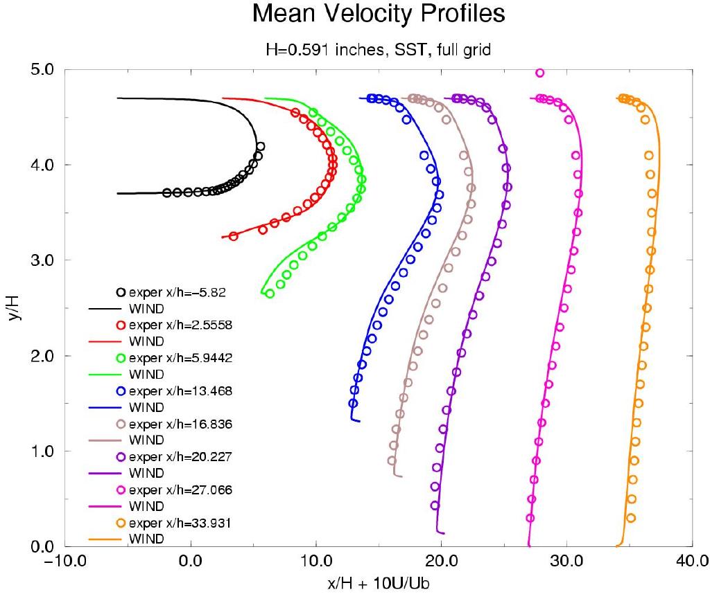
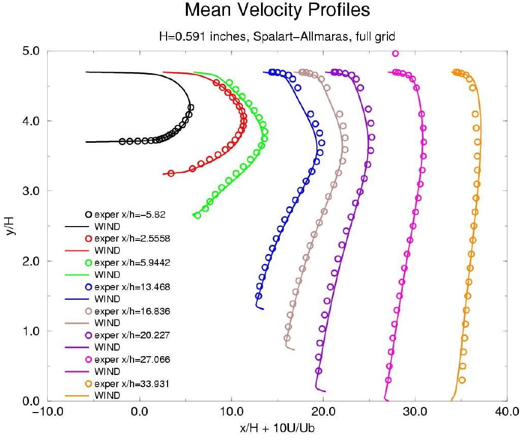
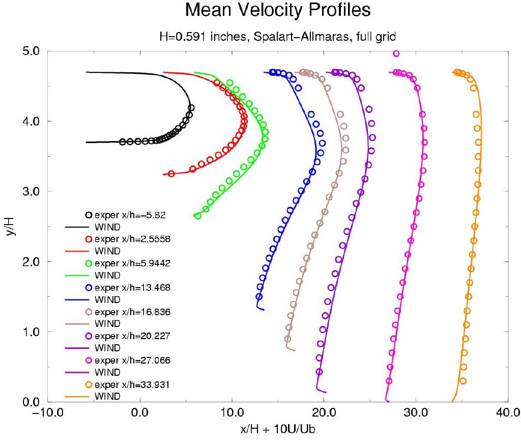
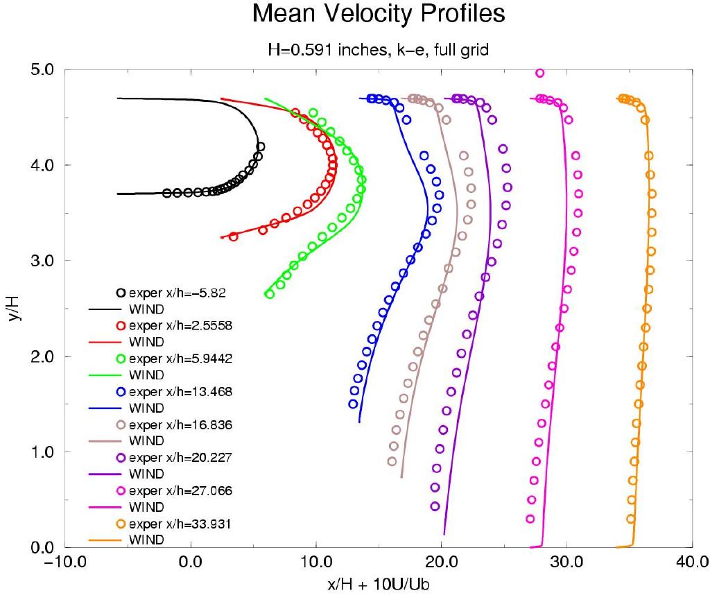
Axial velocity contours (u-component of velocity) for the SST solution are shown in Figure 3. The S-A and k-e solutions gave similar quallitative results and are not shown here. Mean velocity profiles vs experimental data are shown in Figure 4 for different stations downstream (left to right) for the SST, S-A with curvature correction ON, S-A with curvature correction OFF, and k-e models. Both axis are normalized by the inflow height H (0.591 inches). Curve #1 (to the far left in each of the images) represents the fully developed channel flow. The downward slope of the diffuser ramp starts at x/H of 0. The separation region can be seen in Figure 5.
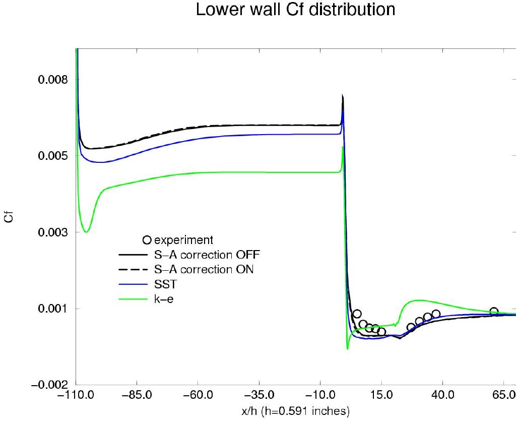
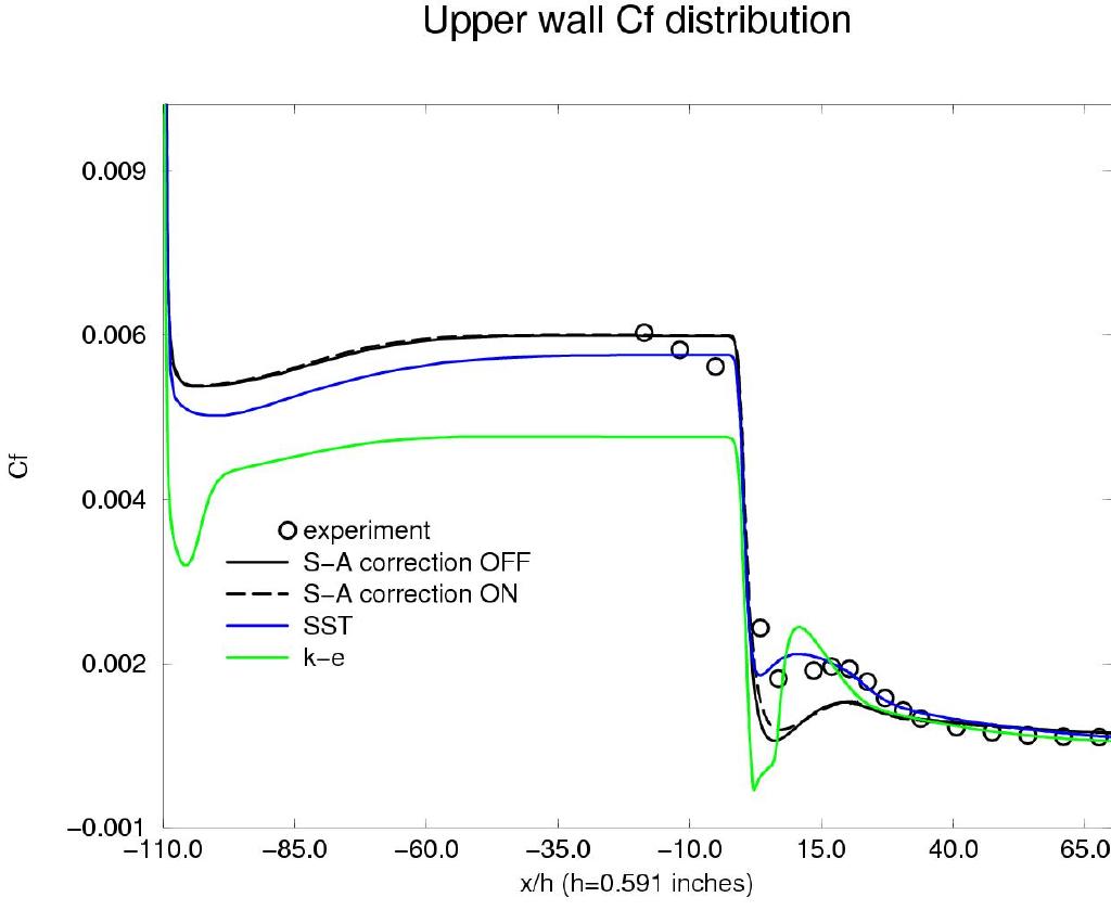
Figure 6 shows the lower and upper wall skin friction vs experimental data on the fine grid for all models. Analysis of the WIND's skin friction coefficient indicates that separation starts at an x/H of 1.9168, and the flow appears to reattach at an x/H of 30.67934 for the SST model. Separation starts at an x/H of 4.0377, and the flow appears to reattach at an x/H of 32.680 with the Spalart-Allmaras rotation correction OFF. Separation starts at an x/H of 3.6051, and the flow appears to reattach at an x/H of 33.044 with the Spalart-Allmaras rotation correction ON. The S-A solution with the curvature correction ON is not significantly different than with it OFF, other than the correction slightly improves the solution on the upper wall near an x/H of 0. For the Chien k-e model, separation starts at an x/H of 0.7583, and the flow appears to reattach at an x/H of 20.943. The S-A solutions produce a slightly higher Cf value (compared with the SST solution) along the upper wall of the diffuser. It underpredicts Cf at x/H of 0 compared with the SST model.
![]()
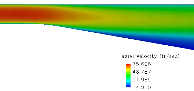
Figure 3. Axial velocity contours (zoomed and unzoomed) for the Buice subsonic 2D diffuser with the SST model. The first image is unzoomed showing the entire computational domain and the second is zoomed near the diffuser ramp area highlighting the separation region.
Figure 4. Axial velocity for experimental data at various stations downstream. From left to right: SST, S-A with curvature correction ON, S-A with curvature correction OFF, and the k-e model.
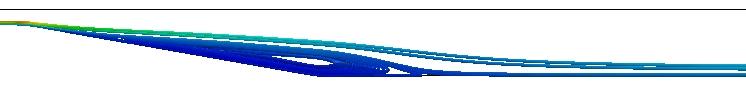
Figure 5. The separation region as highlighted by streamlines for the SST model. The black lines show the upper and lower walls.
Figure 6. Skin friction coefficient along the lower and upper walls of the diffuser vs experimental data.
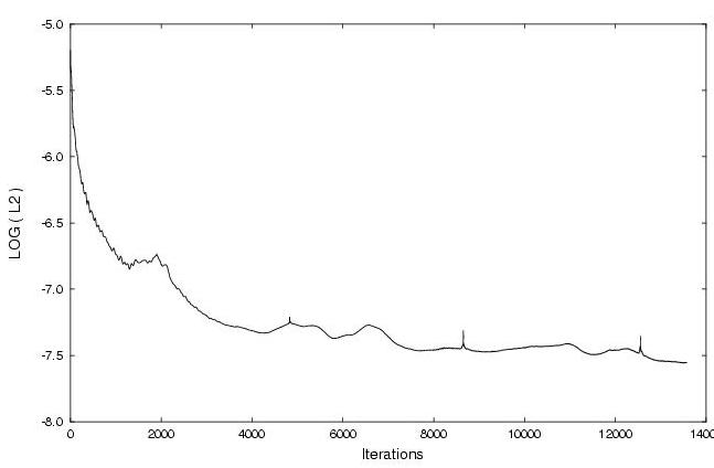
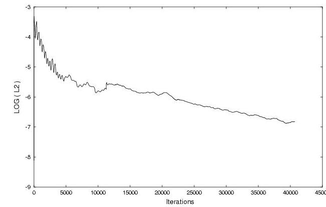
The L2 Norm of the residual for the SST model can be seen in Figure 7. Note that this residual is for the 2nd level grid sequencing (118 axial by 35 vertically). Other grid levels and turbulence models showed similar responses.
Figure 7. L2 Norm of the residual indicating convergence to the steady-state solution. 2nd level sequenced grid for the SST model (left) and fine grid for the k-e model (right).
No sensitivity studies were performed.
The computations were performed on a Silicon Graphics Origin 2000.
Lessons Learned: Conclusions
This solution would not develop properly if the inflow plane boundary condition was “freestream”. Using instead the “arbitrary inflow” produced reasonable results. This was so even when specifying identical inflow conditions. Non-uniform flow properties across the inflow are believed to contaminate the solution when using the Freestream BC for duct flows.
Starting the solution from scratch using the SST model resulted in a very laminar flowfield resulting in too little separation inside the diffuser. This has to do with how SST initializes the flowfield when it starts from scratch. Starting the solution with the S-A model and switching to the SST model solved this problem.
The backpressure (outflow pressure) required at the exit (in order to get nearly the same flow speed just upstream of the diffuser) is dependent on the turbulence model used. The SST model required a higher backpressure than the S-A model. This means that for the same backpressure, the S-A model produced higher flowspeeds through the channel (prior to entering the diffuser).
Qualitative and quantitative results for the S-A and SST models were very similar overall. However, the SST model better predicted the skin friction distribution on the upper wall. The k-e model showed the largest deviations from experiment.
Specifying the massflow at the exit plane resulted in very similar results to specifying the pressure manually using the “downstream pressure” keyword. However, specifying the massflow (if known) eliminates the guesswork for the right backpressure since WIND computes it automatically.
The S-A curvature correction does not significantly alter the results for this problem.
The Chien k-e model failed to predict the separation and reattachment points and proper skin friction profile along the upper and lower walls compared with the S-A and SST models.
Buice, C.U. & Eaton, J.K., "Experimental Investigation of Flow Through an Asymmetric Plane Diffuser”, Journal of Fluids Engineering, Vol. 122, pp. 433-435, June 2000.
Obi, S., Aoki, K., & Masuda, S., “Experimental and Computational Study of Turbluent Separating Flow in an Asymmetric Plane Diffuser,” Ninth Symposium on Turbulent Shear Flows, Kyoto, Japan, August 16-19, 1993, p. 305.
More information on this case can be found at this site or by doing this search in Google. Raw experimental data can be found here.
This study was created on August 11, 2003 by Teryn DalBello, who may be contacted at:
NASA John H. Glenn Research Center, MS 86-7
21000 Brookpark Road
Cleveland, Ohio 44135
Phone: (216) 433-8412
e-mail: teryn@grc.nasa.gov