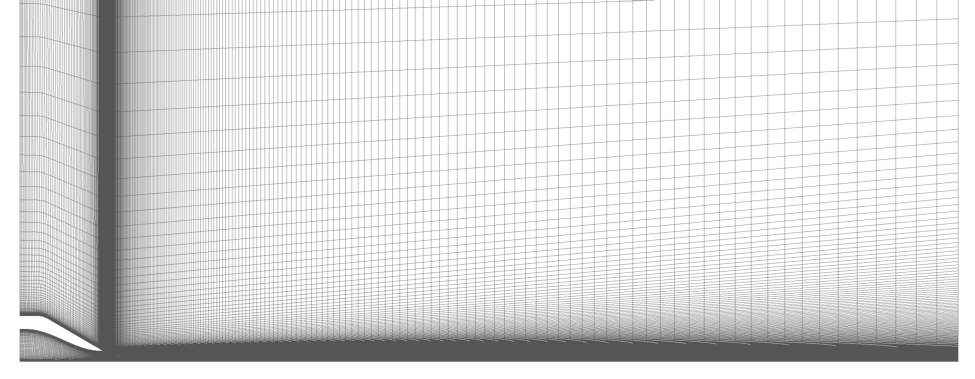
Figure 1. 2-D, structured grid for Acoustic Reference Nozzle.
In this case, unheated flow is passed through convergent nozzle to produce a Mach 0.97 jet flow in quiescent air. The Acoustic Reference Nozzles were developed at NASA Glenn Research Center as a set of reference nozzles for subsonic jet flows for a number of jet acoustic experiments1. ARN2 was used for these studies: it is an axisymmetric, convergent nozzle with a diameter of 2.0 inches. The flow conditions are given in Table 1. The Wind-US simulations presented in this study used a number grids, varied parametrically, in a attempt to determind the best practices when creating grids for the unstrucutred solver within Wind-US. While there were no experimental data to compare the Wind-US results to, the results are compared to each other, with the axisymmetric, structured solver case serving as the baseline.
| Mach | Total Pressure (psia) | Total Temperature (deg R) | Angle-of-Attack (deg) | Angle-of-Sideslip (deg) | |
|---|---|---|---|---|---|
| Jet Inflow | N/A | 26.612 | 529.64 | 0.0 | 0.0 |
| Freestream | 0.01 | 14.3 | 529.63 | 0.0 | 0.0 |
A TAR file containing all the files (grids, solutions, results) for cases presented here is available for download. To unpack the files, use the command:
tar -xvf ARN.tz
| Wind-US 3.153 |
|---|
| ARN.tz |
Since the Acoustic Reference Nozzle is axisymmetric, a 2-D, structured grid was created to be run in axisymmetric mode; it is pictured in Figure 1. The grid consisted of a nearly 60,000 nodes. The nozzle portion consisted of the 121 points in the axial direction and 81 points in the radial direction. The grid points were clustered radially at the nozzle inner wall (to a nominal grid spacing of y+=1) and the centerline.
Figure 1. 2-D, structured grid for Acoustic Reference Nozzle.
Several 3-D versions of the structured grid were created and saved in unstructured format to be run with the Wind-US unstrucutred solver. In general, the strtctured, 2-D grid was extruded in the azimuthal direction. Because Wind-US unstrucuted solver does not allow collapsed boundaries, such as the boundary created along the centerline when a 2-D grid is extruded azimuthally, several schemes were used to grid the region near the centerline: trianglar prisms, quadilateral prisms, and a 10-cell x 10-cell cartesian grid, all aligned with the centerline. The full details for each strucutured, 3-D grid is listed in Table 3. Figure 2 shows diffences between the centerline grid schemes.
| Name | Azimuthal Width (deg) | Azimuthal Cells | Centerline Scheme | Total Cells |
|---|---|---|---|---|
| Str-Uns_5deg-quad | 5 | 2 | quadrilateral-prisms | 118,040 |
| Str-Uns_5deg-tri | 5 | 2 | triangular-prisms | 118,400 |
| Str-Uns_30deg-tri | 30 | 6 | triangular-prisms | 355,200 |
| Str-Uns_45deg-tri | 45 | 10 | triangular-prisms | 592,000 |
| Str-Uns_60deg-tri | 60 | 15 | triangular-prisms | 888,000 |
| Str-Uns_90deg-tri | 90 | 20 | triangular-prisms | 1,184,000 |
| Str-Uns_90deg-cart | 90 | 20 | 10-cell by 10-cell cartesian grid | 1,148,000 |
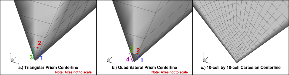
Figure 2. Centerline grid schemes for Acoustic Reference Nozzle Str-Uns grids.
Two unstructured grid were created for the ARN, consisting of rectangles (along the centerline and nozzle wall surfaces) and triangles, extruded in the azimuthal direction. The details of the grids are listed in Table 3, and they are shown in Figures 3 and 4.
| Name | Azimuthal Width (deg) | Azimuthal Cells | Centerline Scheme | Total Cells | Str-Uns_90deg-v1 | 90 | 20 | triangular-prisms | 1,006,847 |
|---|---|---|---|---|
| Str-Uns_90deg-v2 | 90 | 20 | triangular-prisms | 1,957,622 |
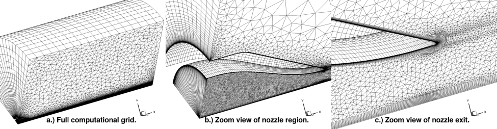
Figure 3. 3-D, unstructured grid for Acoustic Reference Nozzle, grid Uns-Uns_90deg-v1.
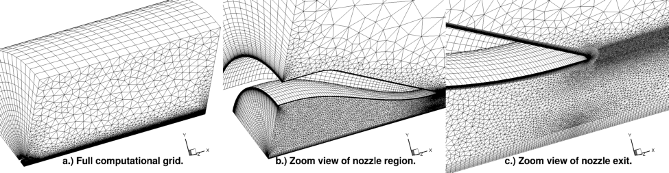
Figure 4. 3-D, unstructured grid for Acoustic Reference Nozzle, grid Uns-Uns_90deg-v2.
After creating the unstructured grids, CFPART was used to create lines in the grid to enable the most efficient use of the unstructured line solver. The grid files and CFPART input files are included in Table 4.
The boundary conditions for this nozzle case are shown in Figure 5. The nozzle and freestream inflows were set to their respective total pressure and total temperature listed in Table 1. The 3-D grids used the inviscid wall boundary condition for the sidewalls. Ideally, these boundaries would have used the connect-coupled boundary condition, to allow for flow in the azimuthal direction, but that was not possible for unstrucutre grids using the grid generation tools publically available at this time. The 2-D grid used the inviscid wall boundary condition along the centerline, which is conventional for 2-D, axisymmetric simulations using Wind-US. In the 3-D grids, the centerline was part of the sidewalls (which are inviscid walls) and did not need to be explicitly set.
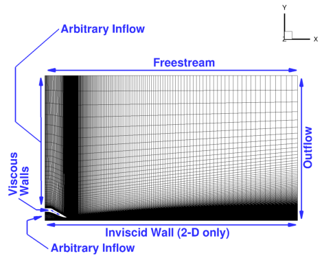
Figure 5. Boundary conditions, shown for the Acoustic Reference Nozzle 2-D, structured grid.
Convergence was determined by monitoring the residuals and two flow field quantities key to this case: the velocity and turbulent kinetic energy along the centerline. The algorithm settings used in the DAT file for these unstructured solver cases are listed in Table 5. Note that settings for the structured solver (i.e., choice of RHS method) were different.
| Field | Str-Str | Str-Uns_5deg-tri | Str-Uns_5deg-quad | Str-Uns_30deg-tri | Str-Uns_45deg-tri | Str-Uns_60deg-tri | Str-Uns_90deg-tri | Str-Uns_90deg-10x10cart | Uns-Uns_90deg-tri-v1 | Uns-Uns_90deg-tri-v2 |
|---|---|---|---|---|---|---|---|---|---|---|
| Version | Wind-US 3.153 | Wind-US 3.153 | Wind-US 3.153 | |||||||
| Grid | 2-D, Structured | 3-D, Structured | 3-D, Unstructured | |||||||
| Solver | Structured | Unstructured | Unstructured | Unstructured | Unstructured | Unstructured | Unstructured | Unstructured | Unstructured | Unstructured |
| Iterations | 35,500 | 50,000 | 55,000 | 10,100 | 10,100 | 10,100 | 10,100 | 10,100 | 10,100 | 16,000 |
| Convergence Order | 9 | 9 | 9 | |||||||
| Method | Default | IMPLICIT UGAUSS LINE EXACT_LHS VISCOUS JACOBIAN FULL CONVERGE FREQUENCY 11 SUBITERATIONS 6 | IMPLICIT UGAUSS LINE EXACT_LHS VISCOUS JACOBIAN FULL CONVERGE FREQUENCY 11 SUBITERATIONS 6 | |||||||
| CFL | 1.0 | AUTO DECREASE 2 CFLMAX 20, CFL# SECONDS 4e-6 |
AUTO DECREASE 2 CFLMAX 20 | AUTO DECREASE 2 CFLMAX 5 | AUTO DECREASE 2 CFLMAX 2 | |||||
| Limiters | Default | DQ LIMITER ON RELAX 0.5 | DQ LIMITER ON RELAX 0.5 | |||||||
| Dissipation | 2 | TVD BARTH 3.0 | TVD BARTH 3.0 | |||||||
| Boundaries | Default | IMPLICIT BOUNDARY ON | IMPLICIT BOUNDARY ON | |||||||
| RHS | Default | HLLE SECOND, VISCOUS FULL | HLLE SECOND, VISCOUS FACE TANGENT | |||||||
| Gradient | Default | LEAST_SQUARES | LEAST_SQUARES | |||||||
| Turbulence Model | SST | SST | SST | |||||||
| Coupling Mode | Default | AVERAGE | AVERAGE | |||||||
The options from Table 5 were incorporated into the DAT input files. The input files for the standard SST turbulence model cases listed above are found in Table 6. The structured grid, structured solver solutions were sequenced to speed up convergence time and demonstrat grid convergence. The grids were run using every fourth grid point, every second grid point, and every grid point in the axial and radial directions.
| Case | DAT File | Str-Str (2D) | ARN_StrStr.dat |
|---|---|
| Str-Uns_5deg-quad | ARN_StrUns-5deg-quad.dat |
| Str-Uns_5deg-tri | ARN_StrUns-5deg-tri.dat |
| Str-Uns_30deg-tri | ARN_StrUns-30deg-tri.dat |
| Str-Uns_45deg-tri | ARN_StrUns-45deg-tri.dat |
| Str-Uns_60deg-tri | ARN_StrUns-60deg-tri.dat |
| Str-Uns_90deg-tri | ARN_StrUns-90deg-tri.dat |
| Str-Uns_90deg-10x10cart | ARN_StrUns-90deg-10x10cart.dat |
| Uns-Uns_90deg-tri-v1 | ARN_UnsUns-90deg-tri-v1.dat |
| Uns-Uns_90deg-tri-v2 | ARN_UnsUns-90deg-tri-v2.dat |
The axial (u-) velocity and turbulent kinetic energy (TKE) were extracted along the jet centerline. Additionally, the u-velocity and TKE were extracted along at plume cross-sections, located at x=0.0, 0.845841, 1.6694, 2.49761, and 3.2945 feet. Table 7 includes the CFPOST scripts for each set of cases.
| Case | CFPOST Script |
|---|---|
| Str-Str | ARN_StrStr.cfpost.com |
| Str-Uns | ARN_StrUns.cfpost.com |
| Uns-Uns | ARN_UnsUns.cfpost.com |
The solutions from the Wind-US simulations listed in Table 5 are presented in Figures 6-10 below. Plots of velocity contours are shown for all cases in Figure 6. Plots or turbulent kinetic energy contours are shown for all cases in Figure 7. In the Str-Uns 5 degree cases, the region of maximum turbulent kinetic energy (TKE) unphysically extends to the centerline at the end of the jet potential core.
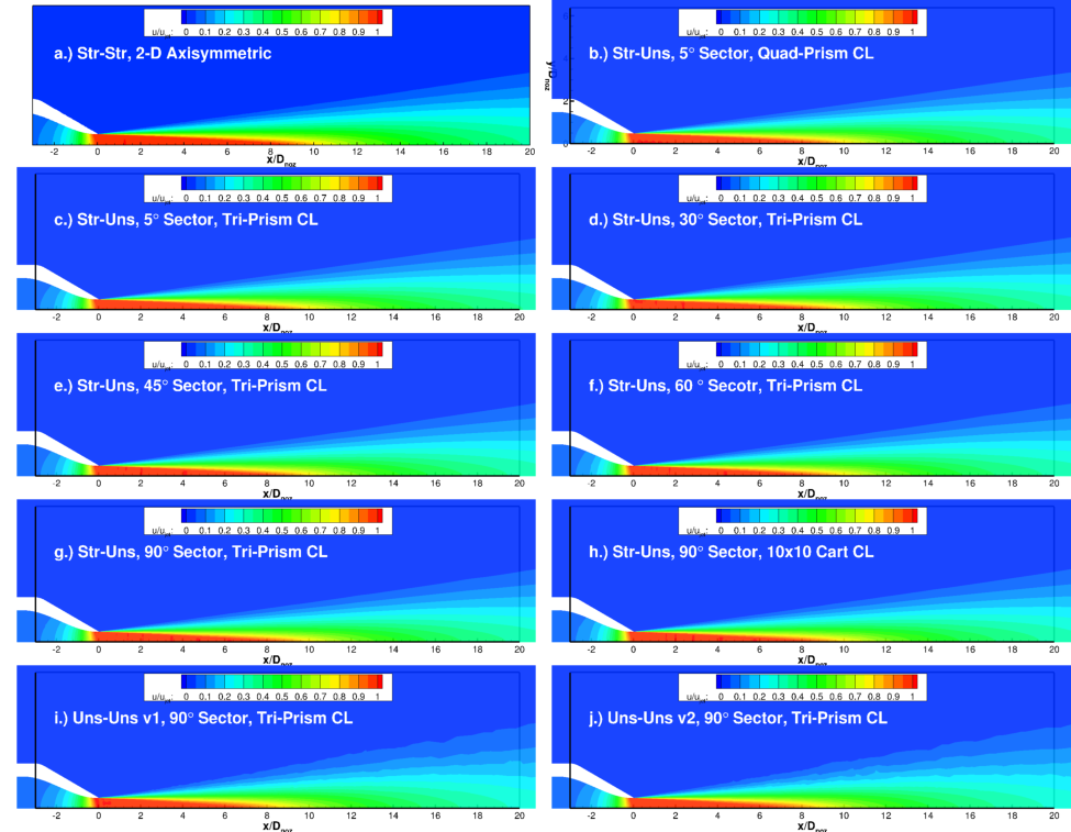
Figure 6. Plots of axial velocity contours.
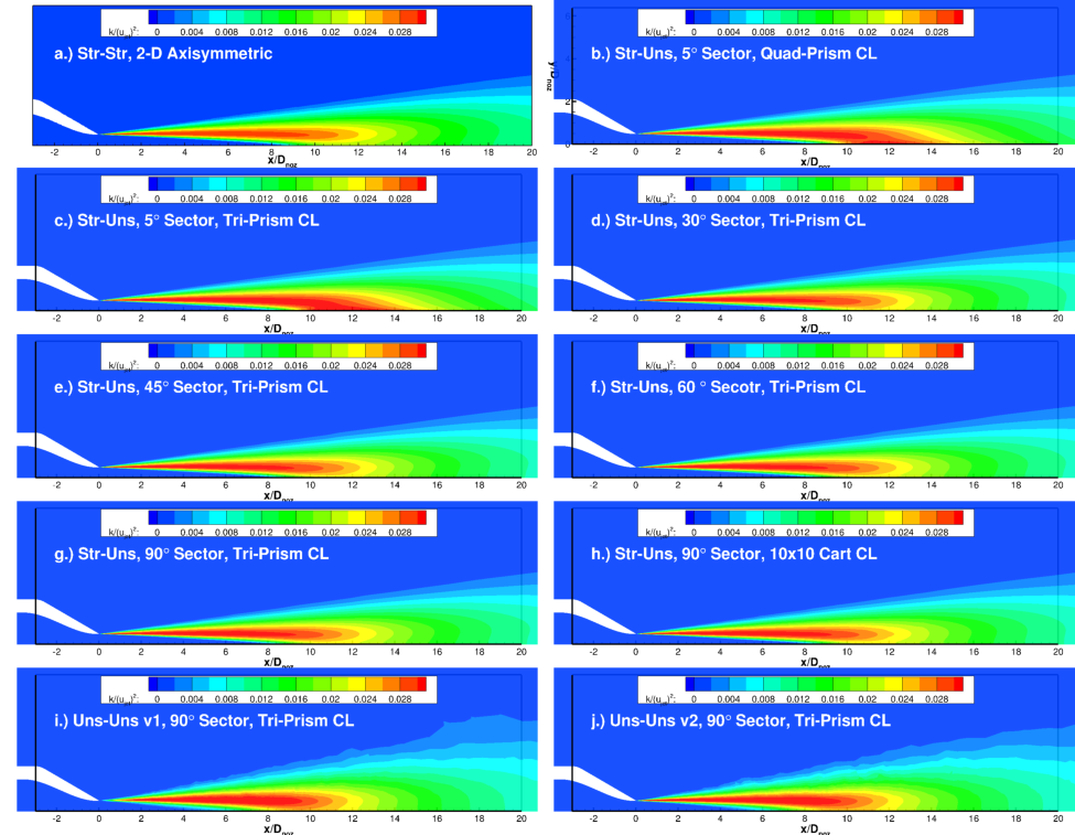
Figure 7. Plots of turbulent kinetic energy contours.
Figure 8 compares the centerline values of axial (u-) velocity and turbulent kinectic energy (TKE) for each grid sequence. Experimental data are also plotted in Figure 8.
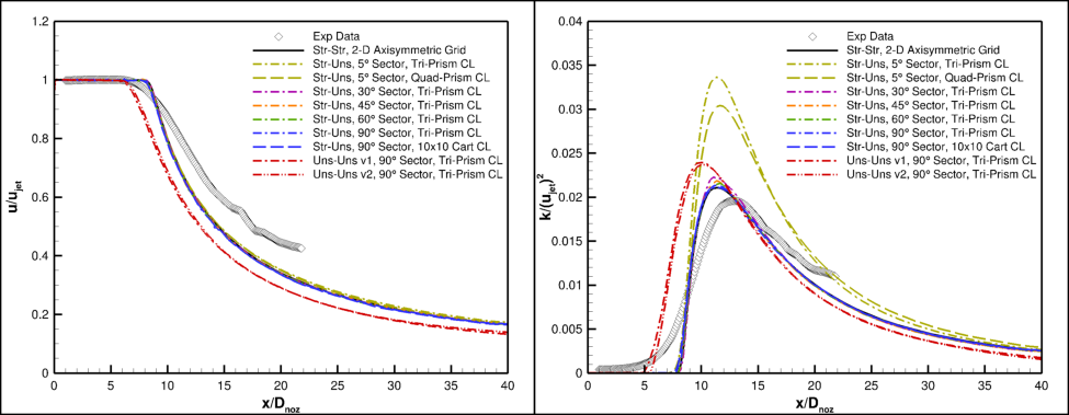
Figure 8. Plot of axial (u-) velocity and turbulent kinetic energy (TKE) along centerline for Acoustic Reference Nozzle simulations.
Most of the simulations (Str-Str and Str-Uns) predict the breakdown of the jet potential core to be several jet diameters downstream of what was observed experimentally. All the simulations predict a larger peak centerline value of TKE and a steeper rate of u-velocity decay than the experimental results.
The Wind-Us simulations can be compared with each other, using the ARN Str-Str case as the reference case. In all of the Str-Uns cases, the jet potential core breaks down around 7.9 jet diameters downstream of the nozzle exit. The 90 degree Str-Uns ARN simulations show excellent agreement with the ARN Str-Str case in both the centerline axial velocity plot and the centerline TKE plot; the centerline grid scheme does not seem to affect the end result. As the size of the azimuthal sector is decreased (60, 45, 30 degrees) the peak centerline TKE increases slightly (less than 10%) from that of the the reference case. When the size of the azimuthal sector is reduced to 5 degrees, the peak centerline TKE increases by over 30%.
The Uns-Uns simulations are consistently different from the reference case. The jet potential core breaks down about 6.3 jet diameters downstream of the nozzle exit, earlier than the reference case. The peak centerline TKE is about 20% greater than the reference case. Increasing the grid resolution along the centerline and the jet shear layer from the Uns-Uns v1 grid to Uns-Uns v2 grid seemed to affect the results little.
Axial velocity profiles and turbulent kinetic energy profiles are plotted in Figures 9 and 10. The normalized axial velocity is significantly less for the Uns-Uns cases at x/D>10. The normalized turbulent kinetic energy is significantly greater for the Str-Uns 5 degree sector cases at x/D>10.
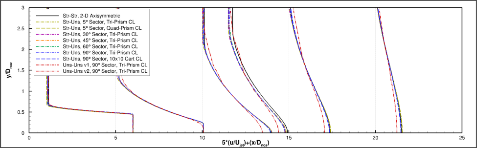
Figure 9. Plot of axial velocity profiles through jet plume.
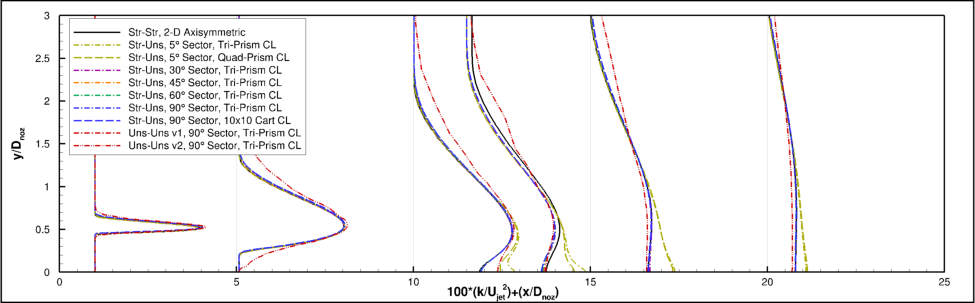
Figure 10. Plot of turbulent kinetic energy profiles through jet plume.
This validation test case was performed by Vance Dippold. Contact: Vance Dippold, MS 5-12, NASA Glenn Research Center, 21000 Brook Park Road, Cleveland, Ohio, 44135.