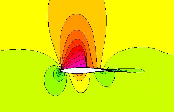
Figure 1. The Mach number contours for the RAE 2822 transonic airfoil.
Figure 1. The Mach number contours for the RAE 2822
transonic airfoil.
This study is an validation study that examines the accuracy of WIND for computing two-dimensional turbulent, transonic flows about an airfoil. The pressure coefficients obtained from the computation from WIND are compared to the values obtained by RAE as reported in Ref. 1. The values obtained from the NPARC validation study are also included in the comparison.
The grid is a single-block, two-dimensional C-grid with dimensions of 369 x 65. It is contained in a PLOT3D grid file named raetaf.x.fmt (formatted, single-zone, 2D, whole). The airfoil surface and wake are located at the J1 boundary. The I-coordinate starts at the lower downstream boundary, intersects the sharp trailing edge at I33, proceeds along the bottom of the airfoil, around the leading edge, downstream along the top of the airfoil, intersects the trailing edge again at I337, and continues to the outflow boundary. The JMAX grid line is the farfield boundary of the flow domain. The grid is non-dimensionalized by the chord length. Since WIND requires dimensional quantities and assumes English Engineering units, the airfoil grid is assumed to have a chord of 1.0 ft. The grid normal to the airfoil surface is clustered about the airfoil surface to resolve the boundary layer on the airfoil. The first grid point off the wall is at a distance of 1.0E-05 ft from the airfoil surface.
The CFCNVT utility is used to convert the PLOT3D grid file to the common grid file format (.cgd) for WIND. This is done using the command
cfcnvt < cfcnvt.x.com
where the file cfcnvt.x.com is a command input file. A common grid file named run.cgd is created. For simulating planar flows in WIND, the three-dimensional flow equations are applied. This requires that the grid plane be in the z = 1.0 plane. The CFCNVT utility creates the proper three-dimensional grid with KMAX = 1.
The boundary conditions must now be specified for the grid and this is done with the GMAN utility. First, the boundary condition types are summarized. A VISCOUS WALL boundary condition is applied at the J1 boundary at the airfoil surface, which extends from I33 to I337. The J1 boundary from I1 to I32 is coupled to the J1 boundary from I338 to IMAX (I369) to form the wake region. An FREESTREAM boundary condition is applied at the JMAX boundary, which should all be subsonic inflow at the freestream conditions. The I1 and IMAX boundaries are specified as OUTFLOW boundaries which allows the static pressure to be directly specified and is assumed to be equal to the freestream pressure.
The boundary conditions can be set either by running GMAN in an interactive mode or by creating an input data file and running GMAN in batch mode. Here the input data file gman.com was created and GMAN was executed as
gman < gman.com
The computation is performed using the time-marching capabilities of WIND to march to a steady-state (time asymptotic) solution. Local time stepping is used at each iteration. The time-marching is performed until iterative convergence is achieved. The convergence criteria was the lift and drag integrated over the airfoild surface.
The input data file is read by WIND at startup to provide WIND with information on performing the simulation. Two different input data files are available that differ by choice of turbulence models. The input data file run.sa.dat uses the Spalart-Allmaras turbulence model. The input data file run.sst.dat uses the SST turbulence model. The freestream keyword indicates that the static freestream flow conditions are specified as Mach number, pressure (psia), temperature (R), angle-of-attack (degrees), and angle-of-sideslip (degrees) as listed in Table 1. The downstream pressure keyword indicates that the freestream static pressure is to be used at the OUTFLOW boundaries. The turbulence model keyword indicates which urbulence model is to be used. The implicit boundary keyword indicates that implicit boundary conditions are applied on the viscous walls. The dq limiter keyword indicates that changes in the solution over an iteration are limited in order to avoid instabilities due to large transients. The loads keyword indicates that the lift on the airfoil is to be integrated every 10 iterations and displayed in the list file. This will be used to evaluate the convergence of the solution. The converge order keyword indicates that the computation will stop if the L2 norm of the solution drops by 9 orders-of-magnitude. The cycles keyword indicates that 500 cycles will be run. The iterations per cycle keyword indicates that 10 iterations will be run per cycle and residual information will be written to the output list file every 5 iterations. The cfl keyword indicates that a CFL number of 5.0 will be used. By default, WIND uses local CFL number to determine the time-step size.
This study assumes freestream flow conditions as summarized in Table 1 below. These conditions correspond to a Reynolds number of 6.5 million based on the chord length of 1.0 ft. The static pressure was computed based on the specified Reynolds number and Mach number and an assumed value of static temperature.
| Mach number | Static Pressure (psia) | Temperature(R) | Angle-of-Attack (deg) |
|---|---|---|---|
| 0.729 | 15.80734 | 460.0 | 2.31 |
The computational flow field is initialized with uniform flow corresponding to these freestream conditions.
The WIND solver is run by invoking the wind script. Further details and options for the wind script can be found in the WIND documentation (wind script).
As WIND runs, an output list file is created which contains the output from the computation and lists the residual information for both the flow equations and the turbulence model equations for each iteration. The integrated lift is also output every 10 iterations.
The output list files for the runs with the Spalart-Allmaras and SST turbulence models are run.sa.lis and run.sst.lis, respectively.
The flow field solution at the final iteration is output to the flow data file. The flow data files for the runs with the Spalart-Allmaras and SST turbulence models are run.sa.cfl and run.sst.cfl, respectively.
There are several ways to examine the convergence of the solution. The RESPLT utility is used for these to read information from the output list file (*.lis). First the L2 norm of the residual of the conservation variables (change over a time step) can be read from the list file,
resplt < resplt.nsl2.com
The file resplt.nsl2.com is a command file containing the inputs for RESPLT to output the GENPLOT formatted plot data file named nsl2.gen of the residuals as a function of the iterations. This file can be plotted using CFPOST,
cfpost < cfpost.nsl2.com
where the file cfpost.nsl2.com is a command file containing the inputs for CFPOST. Fig. 2 shows the solution residual that is displayed by CFPOST.
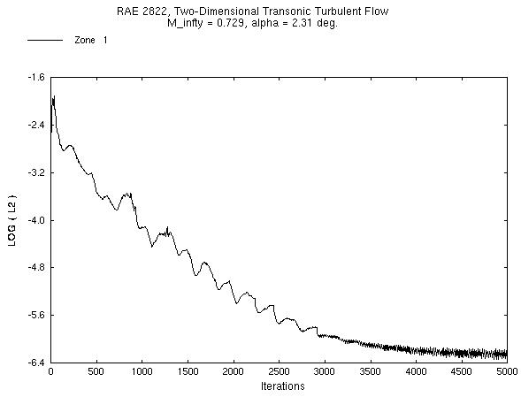
Figure 2. Plot of the L2 solution residual history.
The convergence information for the Spalart-Allmaras turbulence variable can be obtained from the list file using RESPLT,
resplt < resplt.sal2.com
The file resplt.sal2.com is a command file containing the inputs for RESPLT to output the GENPLOT formatted plot data file named sal2.gen of the residuals as a function of the iterations. This file can be plotted using CFPOST,
cfpost < cfpost.sal2.com
where the file cfpost.sal2.com is a command file containing the inputs for CFPOST. Fig. 3 shows the turbulence residual that is displayed by CFPOST.
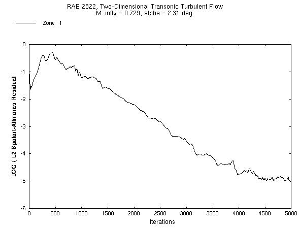
Figure 3. Plot of the L2 turbulence residual history.
A more significant indicator of solution convergence is to examine the convergence of the engineering quantity to be obtained from the analysis. Here it is lift and drag on the airfoil. The loads keyword in the input data file outputs this information into the output list file. RESPLT is used to read this information and create plot files,
resplt < resplt.liftconv.com
The file resplt.liftconv.com is a command file containing the inputs for RESPLT to output the GENPLOT formatted plot data file named liftconv.gen of the residuals as a function of the iterations. This file can be plotted using CFPOST,
cfpost < cfpost.liftconv.com
where the file cfpost.liftconv.com is a command file containing the inputs for CFPOST. CFPOST will display in sequence the plots for drag, lift, and z-direction force. Fig. 4 and 5 shows the convergence of the drag and lift as displayed by CFPOST.
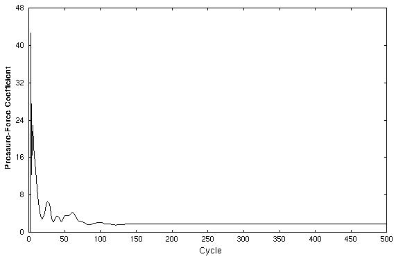
Figure 4. Convergence of the sectional drag on the airfoil
with iterations.
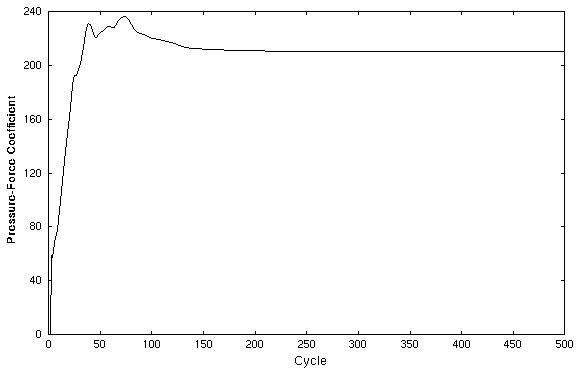
Figure 5. Convergence of the sectional lift on the airfoil
with iterations.
The CFPOST utility can be used to generate engineering information from the the data files.
PLOT3D Files. The PLOT3D files can be obtained using CFPOST
cfpost < cfpost.plot3d.com
The PLOT3D grid and solution files created are named run.x and run.q, respectively. Both are unformatted, whole, 3D, and single-block.
Mach Number Contours. A contour plot of the Mach number about the airfoil as shown in Fig. 6 can be generated using CFPOST
cfpost < cfpost.mach.com
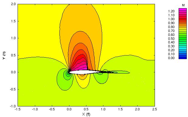
Figure 6. The Mach number contours near the RAE 2822
transonic airfoil.
Static Pressure Contours. A contour plot of the static pressure about the airfoil as shown in Fig. 7 can be generated using CFPOST
cfpost < cfpost.pres.com
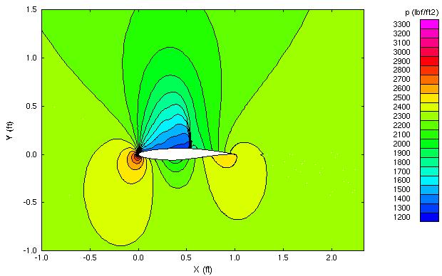
Figure 7. The static pressure contours near the RAE 2822
transonic airfoil.
Pressure Coefficients On the Airfoil. For an airfoil calculation, one piece of important information is the distribution of pressure coefficients on the airfoil. CFPOST can directly output and plot this information,
cfpost < cfpost.cp.com
where cfpost.cp.com is the command input file for CFPOST. A GENPLOT file named cp.wind.gen is created and plotted. The pressure coefficient is negative for pressures less than freestream, which occurs on the top of the airfoil. In plots of pressure coefficients for airfoils, the negative of the pressure coefficient is usually plotted to indicate that the lower pressure region is on the top of the airfoil and the high pressure region is on the bottom of the airfoil. This is done in the CFPOST command file cfpost.cp.com.
Pressure coefficient data from a wind tunnel experiment is available for comparison and is in the GENPLOT file cp.exp.gen.
Figure 8 presents the comparison between the experimental data and WIND. Reference 1 indicates that the experimental error in measuring the static pressure coefficient was approximately 0.0026. This small of error is much smaller than the circle representing the data point, and so, is not plotted. The "WIND" results plotted are those obtained using the Spalart-Allmaras turbulence model. Also plotted are the results from earlier computations using the NPARC code, which are contained in the GENPLOT file cp.nparc.gen.
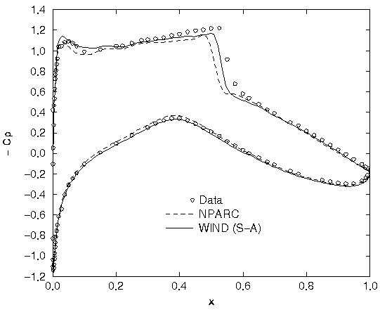
Figure 8. Plot of the pressure coefficients on the airfoil.
Airfoil Forces. For an airfoil calculation, another piece of important information is the forces on the airfoil which result from pressure and skin-friction. CFPOST can be used to integrate these forces over the surface of the airfoil,
cfpost < cfpost.forces.com
where cfpost.forces.com is the command input file for CFPOST. A list file named forces.lis is created in which the force information is printed.
Skin Friction Coefficients On the Airfoil. The skin friction coefficients along the surface of the airfoil can be computed,
cfpost < cfpost.cf.com
where cfpost.cf.com is the command input file for CFPOST. A GENPLOT file named cf.wind.gen is created in which the skin friction coefficients are listed.
Boundary Layers. For a viscous computation, it is useful to examine how well the boundary layers were resolved. One measure of this is the y+ values at the grid points in the boundary layers. The list file forces.lis does contain information on the y+ values throughout the grid. The analysis indicates that the average y+ value of the first point off the wall is less than 2.0. To examine the boundary layer at a certain location, CFPOST can be used.
cfpost < cfpost.blan.com
The file cfpost.blan.com is a command file which writes out the x and y coordinates, u-velocity, v-velocity, and temperature at I250, which is on the top of the airfoil just before the trailing edge blan.gen.
Figure 8 shows the comparisons of the computed surface pressure coefficients with NPARC and experimental results. The WIND results follow the trend of the NPARC results with a slight improvement in the capture of the shock on the upper surface.
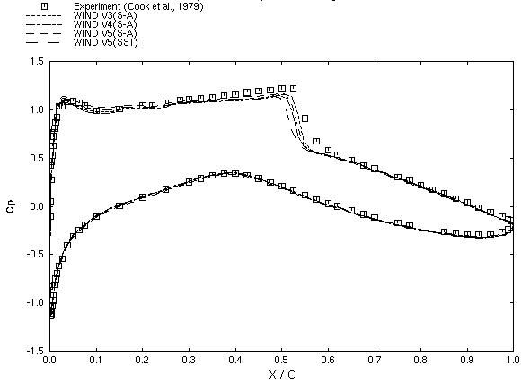
Figure 9. Comparison of static pressure distributions for
the various versions of WIND.
No sensitivity studies were performed.
The computations were performed on a Silicon Graphics Octane using a single R12000 300 MHZ processor. The computation of 500 cycles using version 5.0 with the Spalart-Allmaras turbulence model required 7280 CPU seconds.
Most of the smaller files of this validation case (this does not include the grid, output list, and solution files) are available in the Unix compressed tar file raetaf04.tar.Z. The files can then be accessed by the commands
uncompress raetaf04.tar.Z
tar -xvof raetaf04.tar
1. Cook, P.H., M.A. McDonald, M.C.P. Firmin, "Aerofoil RAE 2822 - Pressure Distributions, and Boundary Layer and Wake Measurements," Experimental Data Base for Computer Program Assessment, AGARD Report AR 138, 1979.
This study was created on May 3, 2002 by John W. Slater, who may be contacted at
NASA John H. Glenn Research Center, MS 86-7
21000 Brookpark Road
Brook Park, Ohio 44135
Phone: (216) 433-8513
e-mail: John.W.Slater@grc.nasa.gov