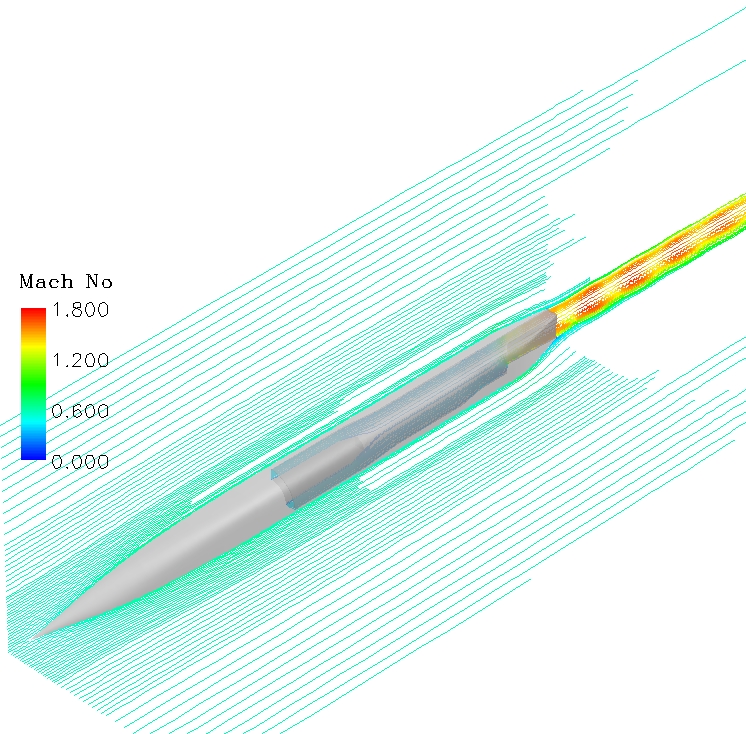
Figure 1. Streamlines for the MADIC 3D Boattail Nozzle. (Note: Some streamlines are shown in 1 zone only.)
Figure 1. Streamlines for the MADIC 3D Boattail Nozzle. (Note: Some streamlines are shown in 1 zone only.)
The problem consists of a three dimensional nozzle body immersed in a M = 0.6 free stream flow at zero angle of incidence. The free stream total pressure is 14.7 psia and the total temperature is 540 deg R. The overall configuration is shown in Figure 1. The nozzle plenum pressure ratio (NPR = Pt,noz/Pinf) is 4.0 and the plenum total temperature is 500 deg R. The free stream Reynolds number is 481000/inch. The data of interest for this case are profiles of pitot pressure ratio (ratio of pitot pressure to free stream total pressure) in the nozzle exhaust plume. The particulars of the test setup and execution from which the data of this study is drawn is found in NASA-TM-88990.
Most of the archive files of this validation case are available in the Unix compressed tar file madic_3d_02.tar. The files can then be accessed by the command:
tar xvof madic_3d_02.tar
NOTE: Because of their large size the following files are not included in the tar file and should be downloaded separately: madic_3d_u.cgd, run1.cfl, and run1.lis. These files should be moved to a directory named run1.
The geometry consists of a sharp nose ogive which transitions into a rectangular nozzle section at the aft end. A detailed elevation view of the test hardware from which the CFD model is derived is given in Figure 2. As in Study 1 the model sting, high pressure plenum and a flow straightener in the downstream converging/diverging (CD) nozzle section are not modeled. The internal nozzle plenum injection ports are also not modeled in this study and due to the symmetry of the geometry, a 90 degree section was modeled with two symmetry planes.
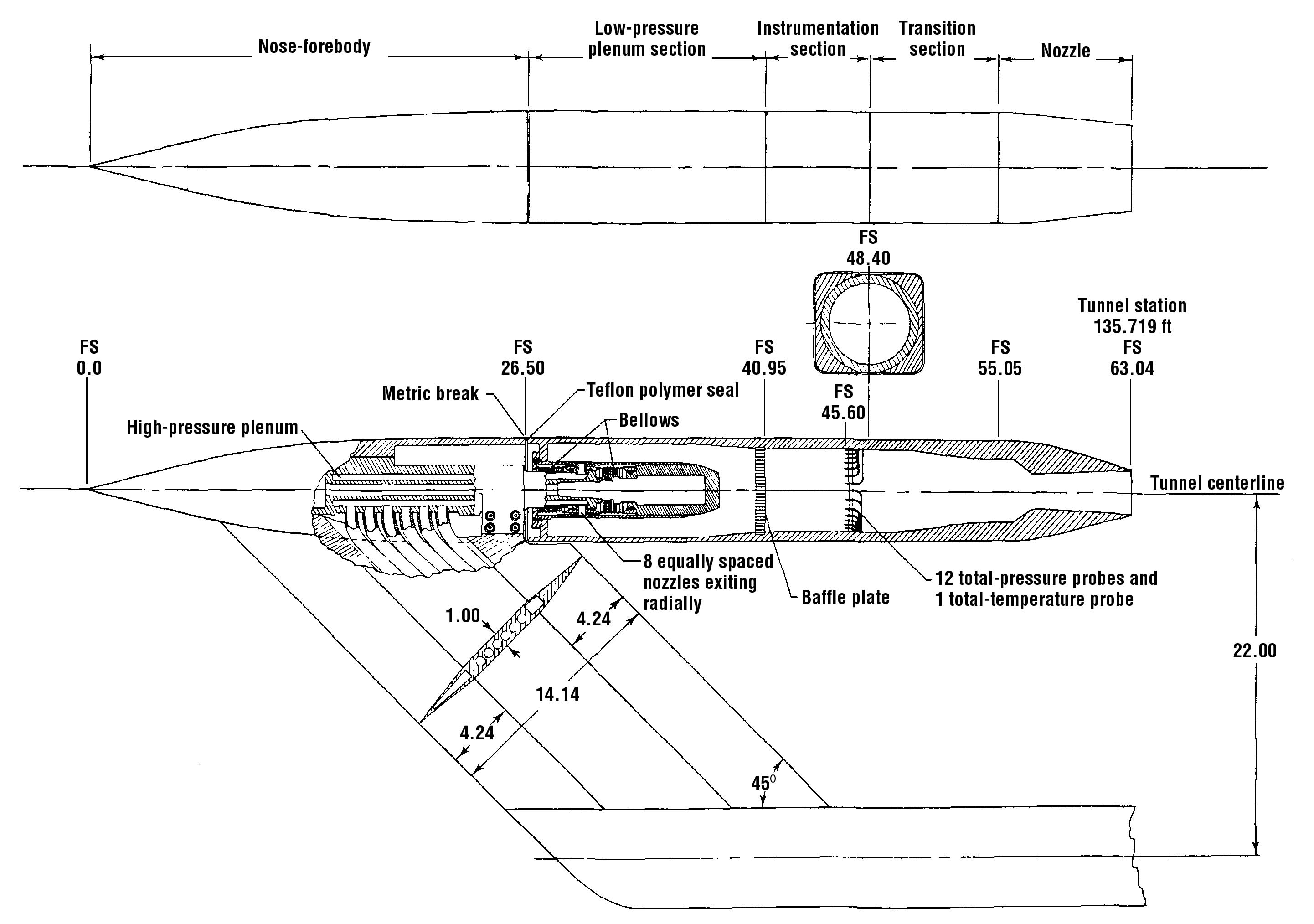
Figure 2. Model Schematic
The initial grid was generated using the AFLR unstructured meshing routines (Ref. 2) along with the Modular Aerodynamic Design Computational Analysis Process (MADCAP) and other Wind-US utilities. Many of details of the grid generation are not available to be included in this document. The grid was initially built in 3 zones: the inner domain of the nozzle, the exhaust plume, and an outer domain grid. (This initial grid is not availabe for downloading.) The nozzle grid was split into two zones as was the exhaust plume. The outer grid was split into 5 zones giving a total of 9 zones, which are described in Table 1, below. The entire grid had about 149,600 volume grid cells.
| Zone | Description | Number of Cells |
|---|---|---|
| 1 | Upstream Nozzle | 14,294 |
| 2 | Downstream Nozzle | 7,169 |
| 3 | Upstream Exhaust Plume | 31,158 |
| 4 | Downstream Exhaust Plume | 19,212 |
| 5 | Upstream Outer Grid | 11,586 |
| 6 | Outer Grid at Instrumentation Section, Transition Section and Nozzle Stations | 14,596 |
| 7 | Outer Grid at Nozzle Stations | 20,511 |
| 8 | Outer Grid at Upstream Plume Stations | 17,979 |
| 9 | Outer Grid at Downstream Plume | 13,129 |
Views of the grids are given in Figures 3 through 6, below.
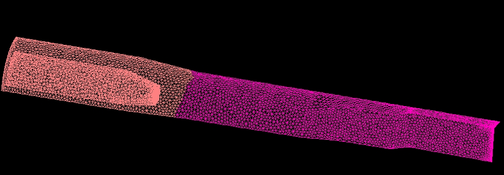
Figure 3. Zones 1 and 2: Internal grid showing viscous wall surfaces on the nose forebody, low pressure plenum, instrumentation section, transition section and nozzle.
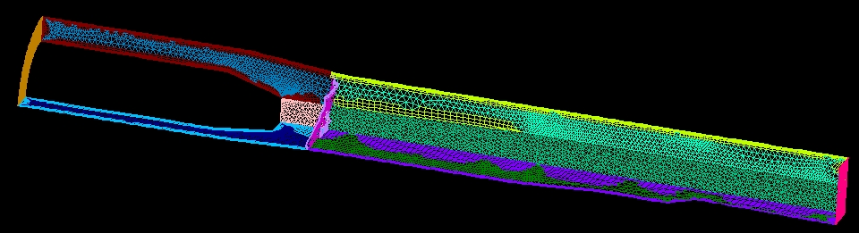
Figure 4. Zones 1 and 2: All boundaries surfaces except viscous walls.
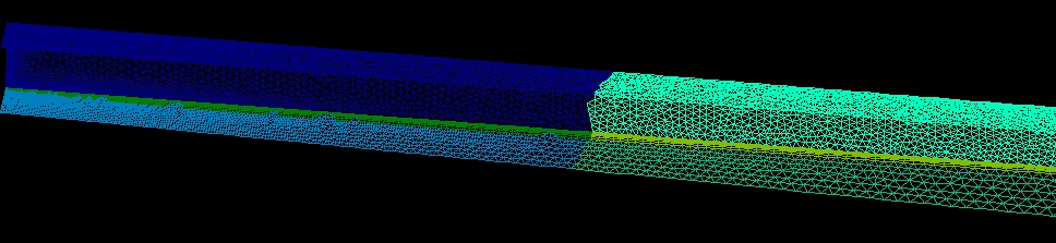
Figure 5. Zones 3 and 4: Exhaust plume.
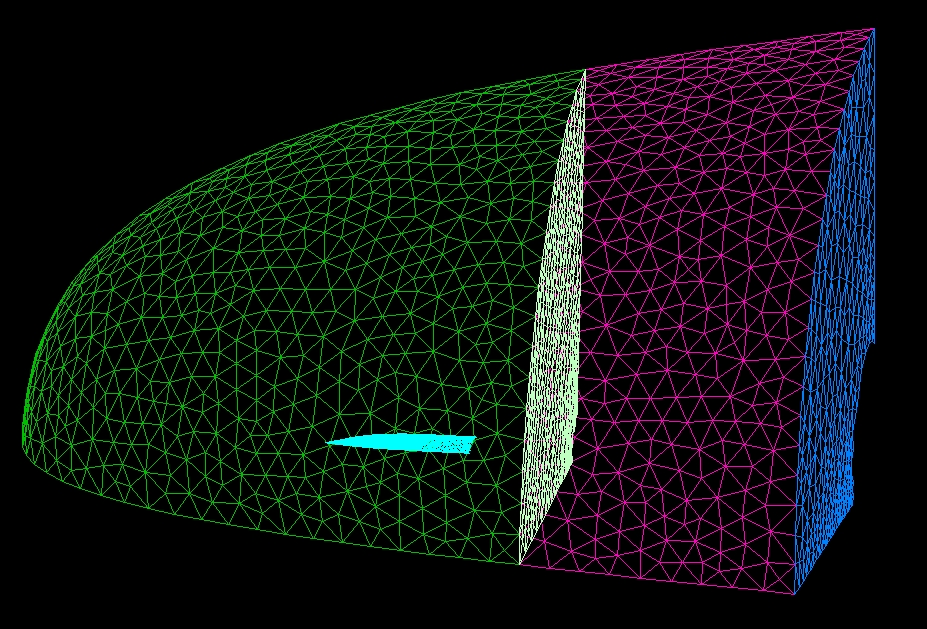
Figure 6. Zones 5 and 8: Outer grids.
All zones had their initial conditions set to free stream values. The free stream total values are given in the following table.
| Mach number | Total Pressure (psia) | Temperature (R) | Angle-of-Attack (deg) |
|---|---|---|---|
| 0.600 | 14.7 | 540.0 | 0.0 |
The boundary conditions were specified previously using MADCAP. The boundary conditions for each zone and respective surface are summarized in the text file bcreport.txt. The VISCOUS WALL boundary conditions on the outer nozzle surface are defined in zones 5 and 6 and on the internal surfaces of zones 1 and 2. INVISCID WALL boundaries are used on the symmetry boundaries throughout every zone, and the COUPLED boundary condition is used for each coupled boundary interface. (Note: The INVISCID WALL boundary condition is identical to the REFLECTION boundary condition.) There are various options available for coupling including regular versus overlapping, tolerance setting, coupling mode, coupling interpolation mode and boundary layer coupling. The details of the coupling were not available to be included in this document.
Even though the boundary conditions have been previously set, you can still use MADCAP to examine them as well as the grid. To do this,
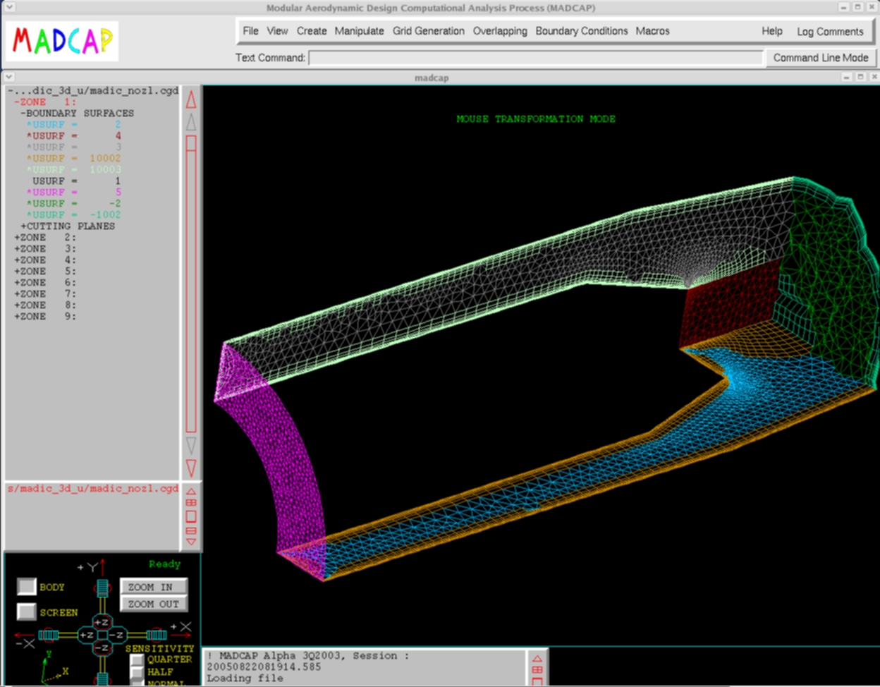
Figure 7. ZONE 1 USURFS displayed in Madcap.
The computation is performed using the time-marching capabilities of WIND-US to march to a steady-state (time asymptotic) solution starting from an initial solution. Local time stepping is used at each iteration to enhance iterative convergence. The Gauss-Seidel implicit operator was specified for further enhancement of the left-hand-side equations. The solution starts marching from the uniform initial conditions which are set to the freestream. The flow is assumed to be fully turbulent. Since the injection ports are not specified as in Study 1, the upstream boundary of the low pressure plenum is set to the conditions given in Table 3 below to mimic the effects of the injection ports.
| Mach number | Total Pressure (psia) | Temperature (R) | Angle-of-Attack (deg) |
|---|---|---|---|
| 0.43 | 46.18 | 500.0 | 0.0 |
This case is computed as a series of runs by placing the wind_post script in the run directory. The input data files are named run1.dat.n where n is the number of the run, from 1-8. For the first run, run1.dat.1 was copied to the file run1.dat. For subsequent runs, the wind-post script copies the file run1.dat.i, where i is the run number to run1.dat. All run1.dat.n files contain the same inputs with the exception of runs 1 and 2 which specify CYCLES 5000, while the remaining runs specify CYCLES 2500. The corresponding output flow files are named run1.cfl.n. Only run1.cfl.8 is included in this distribution.
The FREESTREAM keyword indicates that the freestream conditions are specified as the total values given in Table 2. The TURBULENCE MODEL keyword indicates that the Spalart-Allmaras turbulence model is to be used. The CFL keyword indicates that a number of 1.0 will be used. The ITER_CYCLE keyword indicates that 1 iterations will be performed per cycle and that convergence information will be written to the output list file every iteration. The RHS keyword indicates that the Rusanov 2nd order-upwind cell-centered scheme is used as the right-hand-side explicit operator. The IMPLICIT keyword indicates that the Gauss-Seidel implicit operator is to be used and that the flux Jacobian is to be computed on each face with the Jacobians are saved between iterations. The SMOOTHING keyword specifies that 0.5 is used for the flux dissipation paramater, 1.5 is used for the Jacobian dissipation parameter and 2.5 is used for the slope limiting parameter. The TIMEMARCHING keyword specifies that local time stepping is used with the limit of the maximum to minum time step size set to 108. The DQ LIMITER keyword limits the change in energy to no more than 8% over a single iteration. The Q LIMIT keyword sets limits on the pressure and density to be a maximum of 200 times the freestream value and a minimum of 0.01 times the freestream value in order to aid convergence. The GRID LIMITER keyword specifies that the explicit operator switches to a first order scheme in the presence of grid turning greater that 150 degrees; this helps to reduce numerical instablities near areas with a large amount of grid turning. The ARBITRARY INFLOW keyword block is used to set the inflow conditions on the inflow plane of the low pressure plenum to the total conditions listed in Table 3. The DOWNSTREAM PRESSURE keyword sets the static pressure at the outflow boundaries to 11.52 psi.
The computation was run using Wind-US Version 1.126 on a 2-processor HPXW6200 Linux workstation. The first case was submitted using the wind script with the following options:
wind -runinplace -dat run1 -grid madic_nozl -mp -parallel
This runs the wind script which sets up the computation for the solver. Further details and options for the wind script can be found in the WIND documentation (wind script). A brief description of script options can be listed by typing:
wind -help
The -runinplace option indicates that WIND is to be run in the directory in which the wind script is executed. Otherwise a temporary directory is created for the computation.
The -dat run1 option indicates that the input data file:
run1.dat has the prefix run1.The -mp option indicates that the computation is being performed on a multi-processor computer. The -parallel option is used along with the -mp option to indicate that the computation will be executed in parallel. The parallel computing capability also requires the creation of a multiple processor control file named run1.mpc that includes information on how many processors to use.
As mentioned above, before the first run, the file run1.dat.1 was copied to the file run1.dat. Subesequent runs are submitted automatically using the wind_post script, which was resides in the run directory and copies the correct run1.dat.i file to run1.dat for each run.
The output file run1.lis is generated as the computation proceeds, accumulating the residual information for all iterations. The data flow files run1.cfl.n are generated for each run. Only the flow file for the last run, run1.cfl.8 is included in this distribution.
The convergence properties of the solution are described within the list file (run1.lis), and the data can be extracted by the interactive utility RESPLT. A data file containing the L2 residual history of the Navier-Stokes equations and the Spalart-Allmaras turbulence model (l2.gen) can be generated by:
resplt < resplt.l2.com
The utility CFPOST reads this file to create a data plot.
cfpost < cfpost.l2.com
The command file cfpost.l2.com displays the plots on the screen. The L2 residual plot shows up first. Typing "n" displays the second plot which is the SA residual history. The plots for the convergence history for selected zones are shown in Figures 8 and 9.
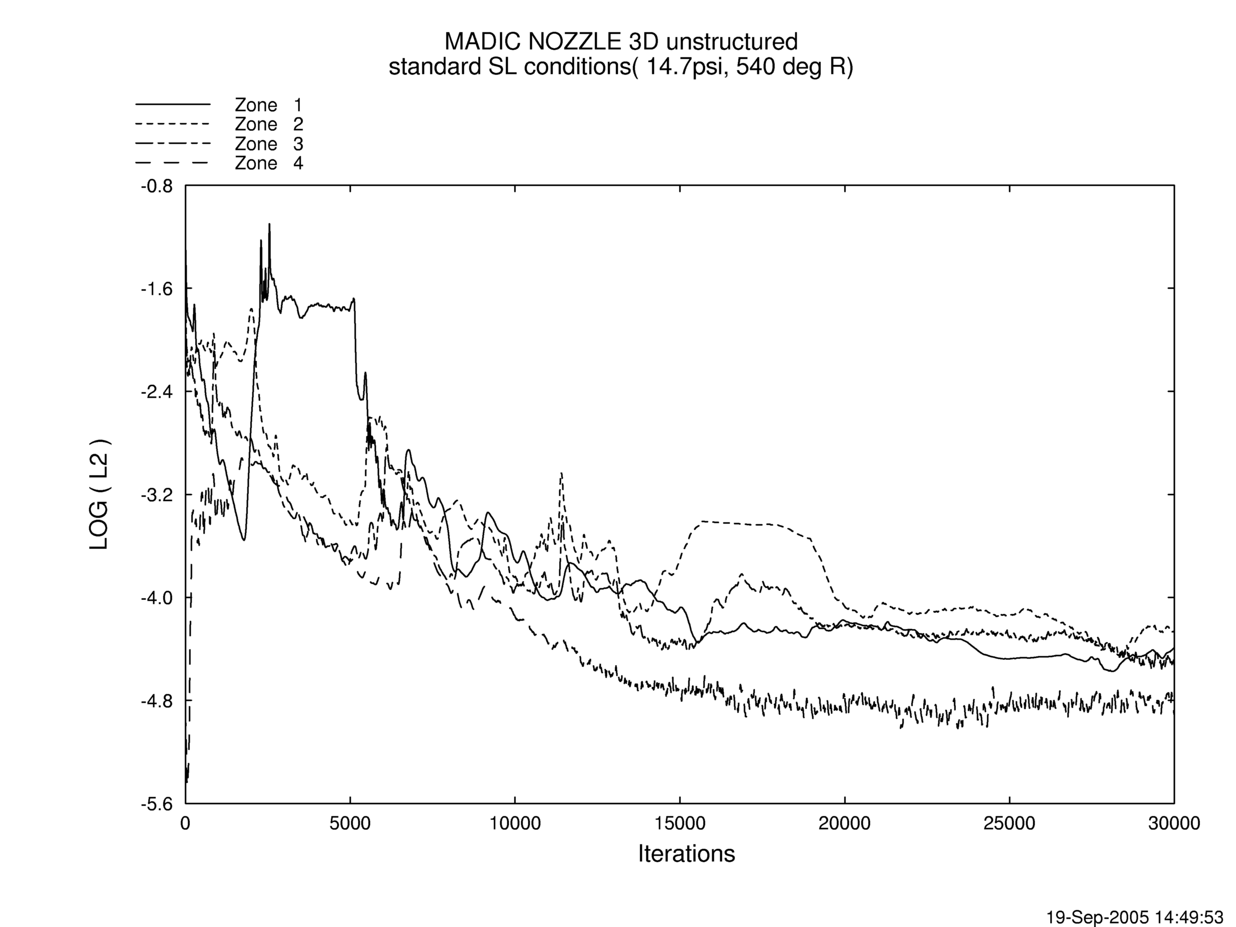
Figure 8. Plot of the L2 solution residual history for the Navier-Stokes equations.
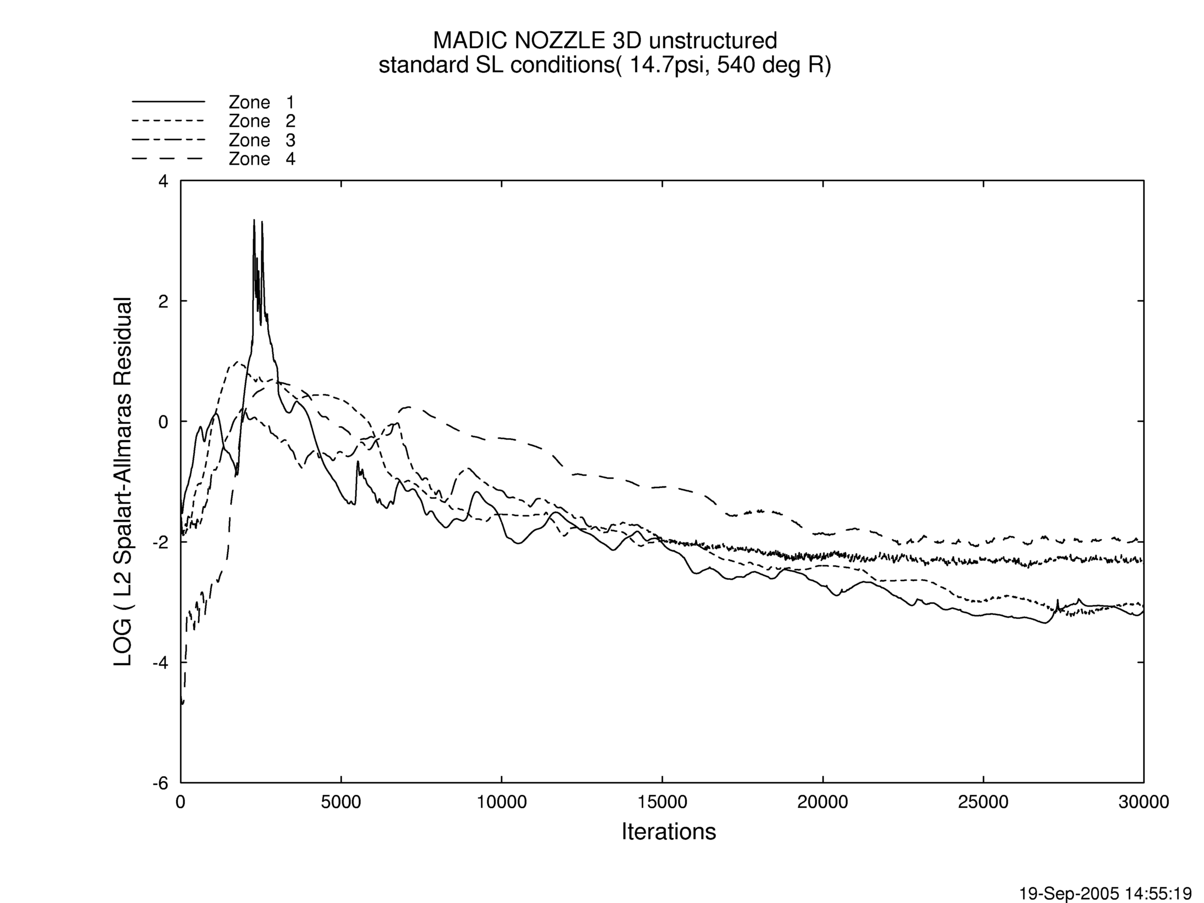
Figure 9. Plot of the L2 solution residual history for the Spalart-Allmaras turbulence model equations.
To visualize the solution, commercial software packages can be used to open and view the .cgd and .cfl files. The pitot profiles shown in Figure 6 were obtained by opening run1.cgd and run1.cfl.8 in a version of the interactive flow visualizer FIELDVIEW compiled with a special Boeing reader. The region of interest is the exhaust plume just downstream of the nozzle exit. The thick blacklines at 0.0, 2.6, 5.1, 7.7 and 10.2 inches from the exit plane of the nozzle indicate the discrete flowfield locations where experimental data exists. The pitot pressures shown are nondimensionalized by the the freestream total pressure which is 14.7 psi.
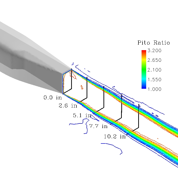
Figure 10. Pitot Pressure Ratio Contours in Exhaust Plume
The pitot pressure profiles in the xy and xz symmetry planes at the five stations shown above were written to separate files using the CFPOST post processing program. CFPOST script files were created to do this. To write the pitot pressure ratio profiles in the xy-symmetry plane, the CFPOST script files cfpost.pitoti_xy.com, were created, where i= 1-5 corresponding to the 5 measurement stations. Similarly, the CFPOST script files to write the pitot pressure ratio profiles in the xz-symmetry plane are named cfpost.pitoti_xz.com. For example, the command:
cfpost < cfpost.pitot1_xy.com
runs CFPOST causing it to write the pitot-pressure ratio values in the xy-symmetry plane at the first station to the file pitotxy1.lis. Similarly, the files pitotxy2.lis, pitotxy3.lis,pitotxy4.lis, and pitotxy5.lis are created for the xy-symmetry plane and the files pitotxz1.lis, pitotxz2.lis, pitotxz3.lis, pitotxz4.lis, and pitotxz5.lis are created for the xz-symmetry plane.
The pitot pressure ratio profiles created above are plotted in the figures 7 and 8 below for the XY and XZ symmetry planes. As can be seen from the data, the WIND results are giving a higher pressure in the core at X = 0.0, 5.1 and 10.2 inches and a thinner thinner shear layer.The disagreement may be due to shortcomings in the turbulence model or to some other physical phenomenon not modeled.
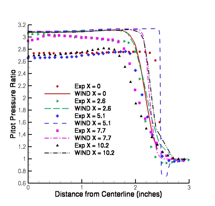
Figure 11. XY Symmetry Plane Pitot Profiles
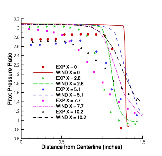
Figure 12. XZ Symmetry Plane Pitot Profiles
The experimental data is listed in Tecplot ASCII "point" format in exp_XY.dat and exp_XZ.dat for the XY and XZ symmetry-planes, respectively. The WIND solution data is similarly listed in wind_XY.dat and wind_XZ.dat, XY and XZ symmetry-planes, respectively. In both experimental and WIND data files, the longitudinal (X) stations are listed as separate Tecplot zones.
According to Reference 1, the estimated instrumentation accuracies are as follows:
| Longitudinal distance X | +/- 0.01 inches |
| Radial distance from center of
rotation of survey probes |
+/- 0.02 inches |
| Roll angle of survey rake | +/- 1.2 degrees |
| Pitot pressure | +/- 0.50 psi |
| Free stream total pressure | +/- 0.0005 psi |
| Free stream total temperature | +/- 0.0005 psi |
| Free stream total temperature | +/- 0.05 R |
| Jet total temperature | +/- 2.5 R |
A repeatability study was conducted in the experiment, and the analysis indicated that the two-standard-deviation (sigma) repeatable band was as shown below for these critical quantities:
| Free stream Mach number | +/- 0.0029 |
| Longitudinal distance | +/- 0.089 |
| Ratio of jet total pressure to
free stream static pressure (NPR) |
+/- 0.034 |
| Ratio of jet total temperature to
free stream total temperature |
+/- 0.030 |
Results from this computation on an unstructured grid may be compared with results from Study1 which was computed on a structured grid.
This case was run using Wind-US version 1.126 on a two-processor HP xw6200 workstation running the LINUX operating system. The computation used approximately 46 sec/iteration of CPU time (23.7 sec/iteration of elapsed time).
1. Putnam, L.E., Mercer, C.E., "Pitot-Pressure Measurement in Flow Fields Behind a Rectangular Nozzle With Exhaust Jet for Free-Stream Mach Numbers of 0.00, 0.60, and 1.20," NASA TM 88990, November 1986.
2. Marcum. D. L.,"Efficient Generation of High Quality Unstructured Surface and Volume Grids", 9th International Meshing Roundtable, Oct. 2000.
This study was created on March 23, 1999 by Michael D. McClure, who may be contacted at
Arnold Engineering Development Center, MS6001
Arnold Air Force Base
Tullahoma, TN 37389-6001
Phone: (931) 454-5826
e-mail: mcclure@hap.arnold.af.mil
The web page was composed by Julianne C. Dudek, who may be contacted at:
NASA Glenn Research Center
21000 Brookpark Road
MS 86-7
Brookpark, OH 44135
e-mail: Julianne.C.Dudek@nasa.gov