
Figure 1. Streamlines for the MADIC 3D Boattail Nozzle.
Figure 1. Streamlines for the MADIC 3D Boattail Nozzle.
The problem consists of a three dimensional nozzle body immersed in a M = 0.6 free stream flow at zero angle of incidence. The free stream total pressure is 14.7 psia and the total temperature is 540 deg R. The overall configuration is shown in Figure 1. The nozzle plenum pressure ratio (NPR = Pt,noz/Pinf) is 4.0 and the plenum total temperature is 500 deg R. The free stream Reynolds number is 481000/inch. The data of interest for this case are profiles of pitot pressure ratio (ratio of pitot pressure to free stream total pressure) in the nozzle exhaust plume. The particulars of the test setup and execution from which the data of this study is drawn is found in NASA-TM-88990.
Most of the archive files of this validation case are available in the Unix compressed tar file madic_3d.tar.Z. The files can then be accessed by the command:
uncompress -c madic_3d.tar.Z | tar xvof -
NOTE: Because of their large size the following files are not included in the tar file and should be downloaded separately: madic_3d.cgd, madic_3d.cfl, madic_3d.dba, madic_3d.gg, and madic_3d.lis.Z.
The geometry consists of a sharp nose ogive which transitions into a rectangular nozzle section at the aft end. A detailed elevation view of the test hardware from which the CFD model is derived is given in Figure 2. The only hardware not modeled are the model sting, high pressure plenum and a flow straightener in the downstream converging/diverging (CD) nozzle section. The internal nozzle plenum consists of 8 circular ports equally spaced around a circular plug. Two planes of symmetry are used in the calculation, requiring only 2 of the port jets to be modeled.
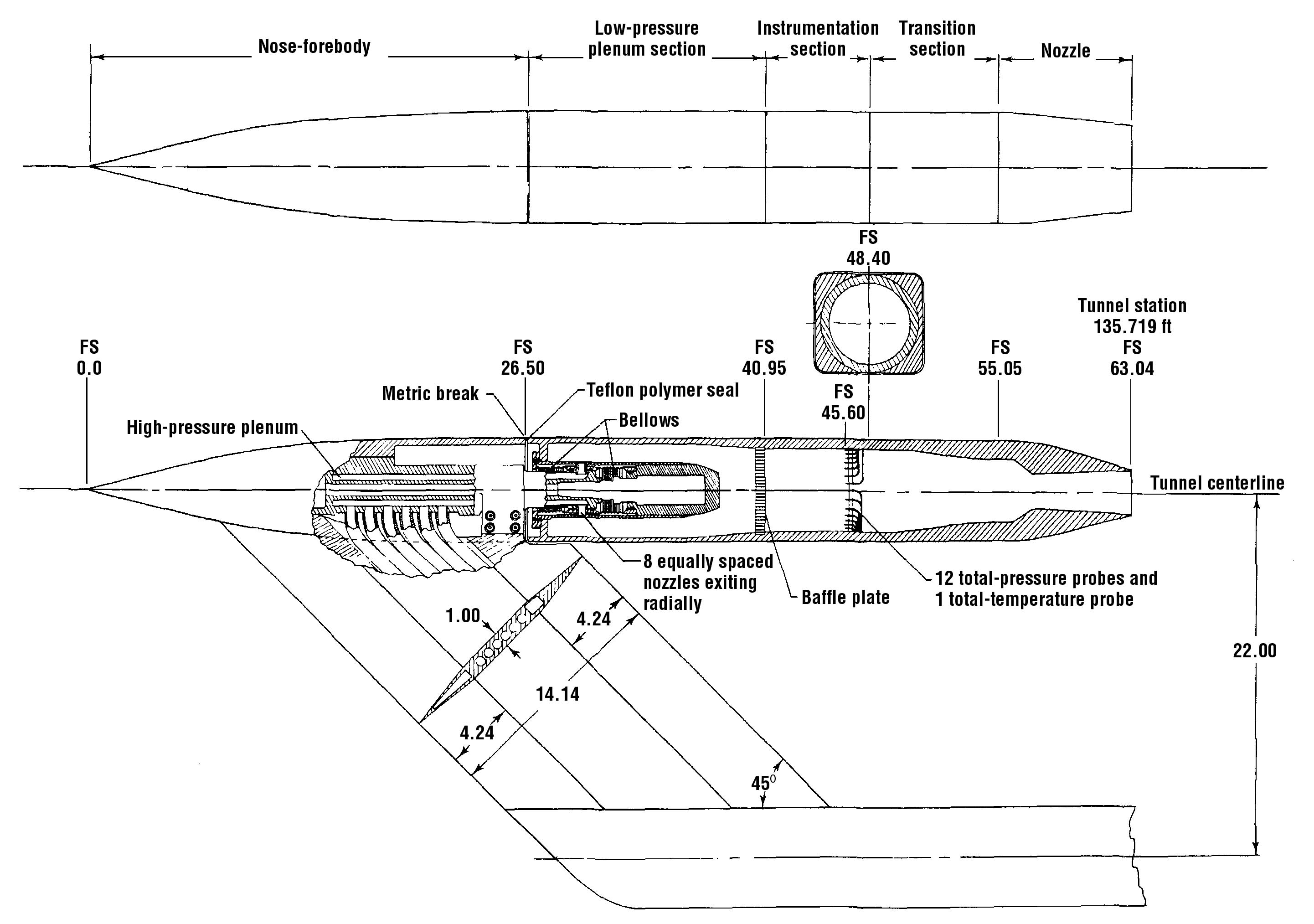
Figure 2. Model Schematic
The initial grid was generated using GRIDGEN (version 13) and consisted of 19 zones and 3.5 million grid points as follows:
1. port_1 73 x 25 x 51
2. port_2 73 x 25 x 51
3. plenum_1 32 x 25 x 101
4. plenum_2 24 x 45 x 101
5. plenum_3 24 x 45 x 101
6. nozzle 65 x 41 x 41
7. nose_1 29 x 46 x 61
8. nose_2 30 x 46 x 61
9. wrap_1 31 x 33 x 61
10. wrap_2 31 x 33 x 61
11. wrap_3 31 x 33 x 61
12. outer_maxy 91 x 15 x 45
13. outer_maxz 91 x 31 x 15
14. plume_1 37 x 104 x 104
15. plume_2 37 x 104 x 104
16. plume_3 37 x 104 x 104
17. plume_4 37 x 104 x 104
18. plume_5 37 x 104 x 104
19. plume_6 37 x 104 x 104
The grid was generated with GRIDGEN, using the database file madic_3d.dba for the solid surface definitions. A majority of the boundary conditions for the flow field solution were defined within GRIDGEN. The output of GRIDGEN is madic_3d.gg. The common file export interface was employed to write out the common grid file madic_3d.cgd for input to WIND.
To facilitate more efficient execution of the problem using parallelism, the last 6 zones were split into 3 zones each using CFSPLIT in the WIND suite of utilities. The final model was made up of 31 zones with the split zones structured as follows.
14a. plume_1a 37 x 67 x 54
14b. plume_1b 37 x 67 x 51
14c. plume_1c 37 x 38 x 104
15a. plume_2a 37 x 67 x 54
15b. plume_2b 37 x 67 x 51
15c. plume_2c 37 x 38 x 104
16a. plume_3a 37 x 67 x 54
16b. plume_3b 37 x 67 x 51
16c. plume_3c 37 x 38 x 104
17a. plume_4a 37 x 67 x 54
17b. plume_4b 37 x 67 x 51
17c. plume_4c 37 x 38 x 104
18a. plume_5a 37 x 67 x 54
18b. plume_5b 37 x 67 x 51
18c. plume_5c 37 x 38 x 104
19a. plume_6a 37 x 67 x 54
19b. plume_6b 37 x 67 x 104
19c. plume_6c 37 x 38 x 104
Views of the grids are given in Figures 3 and 4.
Figure 3. Outer Grids
Figure 4. Nozzle Plenum Grids
All zones had their initial conditions set to free stream values. Zones 1 and 2 had Jameson-type second and fourth order smoothing applied due to strong gradients encountered near the jet shear layers. The smoothing parameters were set to the recommended values in the WIND users manual. The free stream flow values are given in the following table.
| Mach number | Static Pressure (psia) | Temperature (R) | Angle-of-Attack (deg) |
|---|---|---|---|
| 0.600 | 11.525 | 503.7 | 0 |
The first three zones consist primarily of inviscid walls because of the short physical length of these surfaces relative to the JMAX surface, which is set to viscous wall, and due to the extremely low speed (plenum chamber) velocities. The IMAX boundaries in the first two zones are simple point-to-point coupled boundaries to zone 3. On the JMIN surfaces of each zone is a circular H-grid patch which models the normal-jet port with an arbitrary inflow condition. A total pressure of 243 psia and total temperature of 500 deg R are set on these patches and the Mach number is set to unity, designating choked conditions. Zone 3 has JMIN as an inviscid wall and JMAX as a viscous wall. The IMIN and IMAX boundaries are simply coupled to adjacent zones. Zone 4 IMIN is partly a simply coupled boundary and partly an inviscid wall due to the geometry of the backfacing wall of the central plug. IMAX is simply coupled with zone 5 and JMIN is a pinwheel axis boundary. Zone 5 is similar to zone 4 with IMIN simply coupled to zone 4 and IMAX coupled to zone 6 as a chimera boundary due to dissimilar grid topologies in that region. The JMIN and JMAX boundaries are pinwheel axis and viscous wall boundaries respectively. All of the KMIN and KMAX surfaces in zones 1 through 5 are reflection planes with the exception of KMIN and KMAX in zones 2 and 1, respectively, which are simply coupled. The nozzle block, zone 6, is chimera coupled at IMIN to zone 5 and simply coupled to zone 14 on the IMAX end. Boundaries JMIN and KMIN are reflection surfaces and JMAX and KMAX are viscous walls.
Grids 7 through 13 make up the free stream region around the nozzle body. Zones 7 and 8 are polar-cylindrical grids which have the JMAX surfaces set as free stream boundaries as well as the IMIN surface of zone 7. The KMIN and KMAX boundaries are reflection surfaces, and the JMIN boundaries utilize pinwheel axis conditions except for a portion of the JMIN boundary in zone 8. This portion is a viscous wall corresponding to the sharp nose of the nozzle body ogive. Zones 7 and 8 are simply coupled through IMAX and IMIN surfaces, respectively. The IMAX boundary of zone 8 is chimera coupled to zones 9, 12 and 13. Grids 9 through 11 are zones which wrap around the nozzle body outer surface. The IMIN and IMAX boundaries are simply coupled surfaces with the exception of IMIN in zone 9 and IMAX in zone 11; these are chimera coupled to zones 8 and 14, respectively. The JMIN surfaces of these zones are viscous walls and the JMAX surfaces are simply coupled boundaries with zones 12 and 13. The KMIN and KMAX surfaces are reflection surfaces. Zones 12 and 13 extend the domain to the far free stream. They employ H-type grids which interface with zones 8 through 11, as well as 14. The IMIN and IMAX surfaces of both zones are chimera coupled. The JMIN boundary of zone 12 is coupled with zones 9, 10 and 11; JMAX is set to free stream. Zone 12 KMIN is a reflection boundary and KMAX is free stream. Zone 13 JMIN is a reflection surface and JMAX is coupled with zone 12. Zone 13 KMIN is coupled to zones 9 through 11, and KMAX is set to freesteam.
Grids 14 through 19 are the zones encompassing the exhaust plume of the nozzle. The IMIN surface of zone 14 chimera couples with zones 6, 11, 12 and 13. Also, a small portion of that surface is a viscous wall which is the aft backward facing surface of the nozzle exit. The other IMIN and IMAX surfaces of these zones are simply coupled boundaries, with the exception of IMAX in zone 19 which is an outflow boundary. The JMIN and KMIN surfaces of these blocks are reflection surfaces and the JMAX and KMAX are free stream boundaries.
All the boundary conditions are summarized in a table in bcfile.tbl.
Because GRIDGEN already sets a majority of the boundary conditions described above, a quick way of setting the remainder of those conditions is to use GMAN in the batch mode as follows.
gman < gman_19z.com
The file, gman_19z.com, is a command file for GMAN which is configured to set the remaining undefined boundary conditions. The resulting common grid file, madic_3d.cgd, has all boundary conditions set on the 19 existing zones. As mentioned earlier, zones 14 through 19 were split into smaller grids for the purpose of enhanced parallelization. This splitting process begins by copying the first CFSPLIT input file, splt_j67.inp, to the file, fort.1, and then entering the interactive command cfsplit. At the prompt, the input file name (minus the .inp extension) is entered and the unsplit blocks are split at J= 67 . The file, madic_3d_j67.cgd, is created. The process is repeated using the file splt_k54.inp for splitting in the k direction at K= 54, producing a file called, madic_3d_k54.cgd . This file is then copied over the original madic_3d.cgd, completing the process. The CFSPLIT utility not only splits the grids but also splits the associated boundary conditions, relieving the user from setting boundary conditions in the newly created zones.
This problem was executed using the interactive WIND code preprocessor to build and submit a script job file to an ORIGIN 2000. For this example, a solution was generated using a series of runs with the code operating in the parallel mode with 16 processors. The Menter SST Turbulence model was used and the CFL was set to unity. As mentioned earlier, the initial grid was generated using GRIDGEN, and an initial common grid file (.cgd) was written with a majority of the boundary conditions already set. The rest were set using the GMAN utility. The primary control file was generated by the user and contains values of pertinent flow variables related to the solution along with WIND process execution information such as number of cycles to run, CFL number, and turbulence model parameters. A multi-processor control file was also built to specify the number of processors to run in parallel, as well as the frequency to write out the solution file during a run.
The input data file for this WIND example is madic_3d.dat. The free stream keyword is used to set the ambient conditions to those values mentioned in the introduction. The SST turbulence model is specified with the turbulence keyword. An outflow boundary condition is used at the downstream boundary of zone 19 and the keyword downstream pressure is used to set the static pressure to 11.525 psia, consistent with the ambient flow. The arbitrary inflow boundary patches in zones 1 and 2 use the ijk_range keyword to set the jet conditions. The other two files needed are madic_3d.cgd and madic_3d.mpc. The first of these two is the grid and boundary condition file and the second defines the number of processors used per run, along with the frequency of solution file generation.
The WIND flow solver (version 2.0.2.1) was run using the windmp script generator which prompts the user for the job file name root as well as batch queue name. The output file madic_3d.lis is generated as the computation proceeds, accumulating the residual information for all iterations. The data file madic_3d.cfl contains the current solution. As mentioned before, the solution was generated on an SGI ORIGIN 2000 and took approximately 30 cpu seconds per cycle using 16 processors.
The convergence properties of the solution are described within the list file (madic_3d.lis), and the data can be extracted by the interactive utility RESPLT. A data file containing the L2 residual history (madic_3d_res.gen) can be generated by:
resplt < resplt.com
The utility CFPOST reads this file to create a data plot.
cfpost < cfpost.com
The command file cfpost.com displays the plot on the screen and then converts it into a PostScript file (following a Return when the plot appears). The plot for the convergence history for selected zones is shown in Figure 5.
Figure 5. Plot of the L2 solution residual history.
A PLOT3D solution file can be generated using the CFPOST utility as follows.
cfpost < madic_3d_plot3d.com
The command file madic_3d_plot3d.com directs cfpost to write out an unformatted, iblanked, multigrid grid file madic_plot3d.x and a solution file madic_plot3d.q. These files can then be viewed with an interactive flow visualizer such as FIELDVIEW. The region of most interest is downstream of the nozzle exit where experimental data exists. The thick black lines aft of the nozzle exit in Figure 6, generated using FIELDVIEW, illustrates the discrete flowfield locations where experimental and computational values of pitot pressure ratio were compared. To properly normalize the data in the PLOT3D solution file, FIELDVIEW's pitot pressure was multiplied by gamma (= 1.4), the free stream static pressure ( = 11.525 psia) and divided by free stream total pressure (= 14.7 psia). The resulting values were output to separate files for each comparison axial station. The axial locations were at 0, 2.6, 5.1, 7.7, and 10.2 inches from the exit plane of the nozzle.
Figure 6. Pitot Pressure Ratio Contours in Exhaust Plume
The pitot pressure ratio profile plots are given in the figures below for the XY and XZ symmetry planes. As can be seen from the data, the WIND results track within +/- 6% of the level of pitot pressure in the inviscid core region of the plume until the inner edge of the plume shear layer is encountered. At that point, the test data indicates a thicker shear layer as indicated by the divergence of the CFD results from the test data. The disagreement may be due to shortcomings in the turbulence model or to some other physical phenomenon not modeled. Ancillary axisymmetric studies reveal that if the flow straightener is modeled, there is negligible effect on the profile at the nozzle exit.
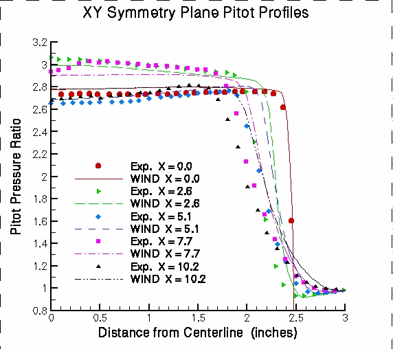
Figure 7. XY Symmetry Plane Pitot Profiles
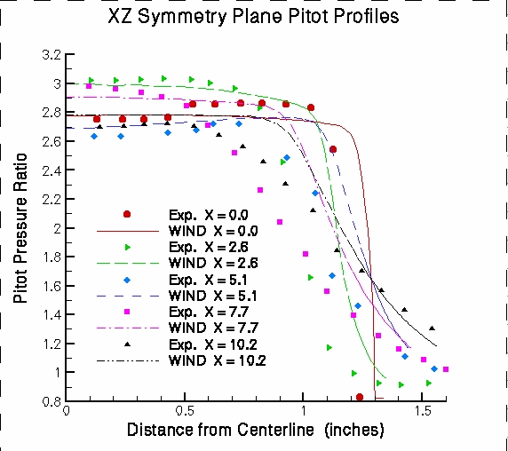
Figure 8. XZ Symmetry Plane Pitot Profiles
The experimental data is listed in Tecplot ASCII "point" format in exp_XY.dat and exp_XZ.dat for the XY and XZ symmetry-planes, respectively. The WIND solution data is similarly listed in wind_XY.dat and wind_XZ.dat, XY and XZ symmetry-planes, respectively. In both experimental and WIND data files, the longitudinal (X) stations are listed as separate Tecplot zones.
According to Reference 1, the estimated instrumentation accuracies are as follows:
| Longitudinal distance X | +/- 0.01 inches |
| Radial distance from center of
rotation of survey probes |
+/- 0.02 inches |
| Roll angle of survey rake | +/- 1.2 degrees |
| Pitot pressure | +/- 0.50 psi |
| Free stream total pressure | +/- 0.0005 psi |
| Free stream total temperature | +/- 0.0005 psi |
| Free stream total temperature | +/- 0.05 R |
| Jet total temperature | +/- 2.5 R |
A repeatability study was conducted in the experiment, and the analysis indicated that the two-standard-deviation (sigma) repeatable band was as shown below for these critical quantities:
| Free stream Mach number | +/- 0.0029 |
| Longitudinal distance | +/- 0.089 |
| Ratio of jet total pressure to
free stream static pressure (NPR) |
+/- 0.034 |
| Ratio of jet total temperature to
free stream total temperature |
+/- 0.030 |
No sensitivity studies were performed.
1. Putnam, L.E., Mercer, C.E., "Pitot-Pressure Measurement in Flow Fields Behind a Rectangular Nozzle With Exhaust Jet for Free-Stream Mach Numbers of 0.00, 0.60, and 1.20," NASA TM 88990, November 1986.
This study was created on March 23, 1999 by Michael D. McClure, who may be contacted at
Arnold Engineering Development Center, MS6001
Arnold Air Force Base
Tullahoma, TN 37389-6001
Phone: (931) 454-5826
e-mail: mcclure@hap.arnold.af.mil