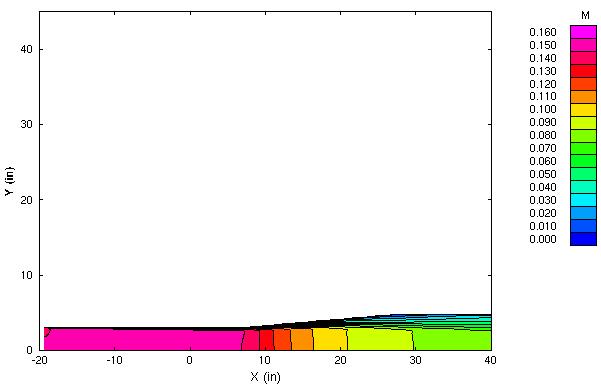
Figure 1. The Mach number contours for the Fraser subsonic conical diffuser.
Figure 1. The Mach number contours for the Fraser
subsonic conical diffuser.
This validation study examines the incompressible, turbulent flow through a conical diffuser.
Most of the files for this study are available in the Unix compressed tar file fraser02.tar.Z. The files can then be extracted by the unix command:
uncompress -c fraser02.tar.Z | tar xvof -
The files fraser.x, fraser.cgd, fraser.cfl, and fraser.lis are not included in order to limit the size of the tar file. They can be downloaded separately.
The grid is contained in a PLOT3D grid file (unformatted, multi-zone, whole, three-dimensional) named fraser.x. It consists a single zone with grid dimensions 121 x 71. The I1 surface is the inflow. The IMAX surface is the outflow. The J1 surface is the axis-of-symmetry. The JMAX surface is the conical diffuser. This grid and the common grid file are identical to those of Study #1. The common grid file is fraser.cgd.
The initial flow conditions are simply the conditions of the freestream keyword as presented in Table 1.
| Mach | Pressure (psia) | Temperature (R) | Angle-of-Attack (deg) | Angle-of-Sideslip (deg) |
|---|---|---|---|---|
| 0.15 | 14.7 | 530.0 | 0.0 | 0.0 |
The I1 inflow boundary is specified with a FREESTREAM boundary condition. The IMAX boundary is specified with an OUTFLOW boundary condition. The J1 boundary is specified with an INVISCID WALL boundary condition. The JMAX boundary is specified with a VISCOUS WALL boundary condition. These are set using GMAN.
The computation is performed using the time-marching capabilities of WIND to march to a steady-state (time asymptotic) solution. Local time stepping is used at each iteration. The time-marching is performed until convergence criteria is achieved.
The WIND input data file for this case is fraser.dat. The freestream keyword indicates that the static freestream flow conditions are specified as Mach number, pressure (psia), temperature (R), angle-of-attack (degrees), and angle-of-sideslip (degrees). The axisymmetric keyword indicates that the axisymmetric flow assumption is used. The turbulence model keyword indicates that the Spalart-Allmaras turbulence model is to be used. The mass flow rate keyword specifies the actual mass flow out the outflow boundary (assuming a 360 degree section). The cycles keyword indicates that a maximum of 3000 cycles will be run. The iterations per cycle keyword indicates that 20 iterations will be run per cycle. The cfl# keyword indicates that a CFL number of 1.3 is used. By default, WIND uses local maximum allowable time-step based on the specified CFL number. The converge level keyword indicates that the computation will stop if the L2 norm of the solution drops to 1.0E-09.
The WIND solver is run by entering:
wind -runinplace -dat fraser
This runs the wind script which sets up the computation for the solver. The runinplace option indicates that WIND is to be run in the directory in which the wind script is executed. The dat option indicates the name of the input data file.
The RESPLT utility is used to read solution convergence information from the list file fraser.lis. First the L2 norm of the residual of the conservation variables (change over a time step) can be read from the list file,
resplt < resplt.nsl2.com
The file resplt.nsl2.com is a command file containing the inputs for RESPLT to output the GENPLOT formatted plot data file named nsl2.gen of the residuals as a function of the number of iterations. This file can be plotted using CFPOST,
cfpost < cfpost.nsl2.com
where the file cfpost.nsl2.com is a command file containing the inputs for CFPOST. Fig. 3 shows the solution residual that is displayed by CFPOST.
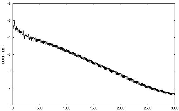
Figure 2. Plot of the L2 solution residual history -vs- cycles.
The convergence of the Spalart-Allmaras turbulence model equation is evaluated b examining the L2 norm of its residual term,
resplt < resplt.sal2.com
The file resplt.sal2.com is a command file containing the inputs for RESPLT to output the GENPLOT formatted plot data file named sal2.gen of the residual as a function of the number of iterations. This file can be plotted using CFPOST,
cfpost < cfpost.sal2.com
where the file cfpost.sal2.com is a command file containing the inputs for CFPOST. Fig. 4 shows the solution residual that is displayed by CFPOST.
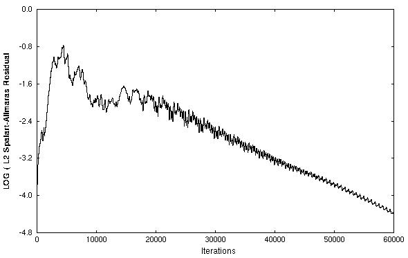
Figure 3. Plot of the L2 norm of the Spalart-Allmaras
turbulence equation residual history.
The CFPOST utility can be used to generate engineering information from the the data files. First, the PLOT3D files can be obtained for displaying in FAST,
cfpost < cfpost.plot3d.com
The PLOT3D solution file created is named fraser.q. It is unformatted, whole, 3D, and multi-zone. The grid file fraser.x is also output.
The CFPOST utility can also be used to generate and plot Mach contours. Fig. 1 shows the Mach contours.
cfpost < cfpost.mach.com
The experiment provides skin friction coefficients along the diffuser wall. These can be obtained from the solution using CFPOST,
cfpost < cfpost.cf.com
where cfpost.cf.com is the command input file for CFPOST to obtain the skin friction coefficients. A GENPLOT file named cf.gen is created and plotted.
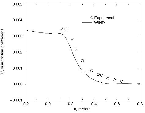
Figure 4. Skin friction coefficients along diffuser surface.
The skin friction coefficients show the similar trend of the experimental data; however, the computed results are lower than the experiment.
No sensitivity studies were performed.
The computations were performed on a Silicon Graphics Octane workstation using a single 300 MHZ IP30 MIPS R12000 Processors. 3000 cycles for 60000 iterations required 22407.50 CPU seconds over an elapsed time of 23252.26 seconds.
Fraser, H.R., "The Turbulent Boundary Layer in a Conical Diffuser," Journal of the Hydraulic Division , Proceedings of the American Society of Civil Engineers, pp. 1684-1-17, June 1958.
This study was created on January 12, 2000 by John W. Slater, who may be contacted at:
NASA John H. Glenn Research Center, MS 86-7
21000 Brookpark Road
Cleveland, Ohio 44135
Phone: (216) 433-8513
e-mail: John.W.Slater@grc.nasa.gov