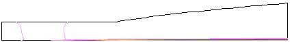
Figure 1. The Mach number contours for a Mach 0.1 flow over a flat plate.
Figure 1. The Mach number contours for
a Mach 0.1 flow over a flat plate.
This validation case is an example case demonstrating the computational process using a simple flow of an incompressible, laminar flow over a flat plate. The results care compared with the analytic results of Blasius.
All of the archive files of this validation case are available in the Unix compressed tar file fplam01.tar.Z. The files can then be accessed by the commands
uncompress fplam01.tar.Z
tar -xvof fplam01.tar
The grid is a single-block, two-dimensional grid generated using the Fortran program fpgrid.f using a streamwise grid spacing of 0.025 and a normal spacing of "eta" of 0.4. The resulting grid density is 51 x 37. A Plot3d file (unformatted, single-block, whole, two-dimensional) named fplam.x.dat was output.
The Plot3d grid file was converted to the common grid file (*.cgd) format using the CFCNVT utility. This was done using the command:
cfcnvt < cfcnvt.x.com
where the file cfcnvt.x.com is a command input file (standard Fortran input unit). A common grid file named fplam.cgd is created.
An initial condition of freestream flow conditions is appropriate for this problem. Here, standard sea level conditions are used:
| Mach number | Static Pressure (psia) | Temperature(R) | Angle-of-Attack (deg) |
|---|---|---|---|
| 0.1 | 6.0 | 700.0 | 0.0 |
These conditions were chosen so that the Reynolds number based on the length of the plate (1.0 ft) was approximately 200000.
A VISCOUS WALL boundary condition is applied at the J1 boundary of the plate, which extends from i=11 to IMAX. An INVISCID WALL boundary condition is applied from i=1 to i=10. AN INFLOW OUTFLOW boundary condition is applied at the I1 boundary since subsonic flow in coming into the flow domain. The IMAX outflow boundary is specified to be a CONFINED OUTFLOW boundary. An INFLOW OUTFLOW boundary condition could also be applied, but the CONFINED OUTFLOW allows the static pressure to be directly specified and we know that it should be equal to the freestream pressure. The farfield boundary at JMAX is placed well above the boundary layer and is a subsonic inflow boundary, and so, it can be specified with a INFLOW OUTFLOW boundary condition.
The boundary conditions are specified using GMAN. The procedure using the graphics interface is as follows:
gman
file fplam.cgd
units fss
swi
Pick SHOW (upper right panel)At this point the grid will be displayed since there is only one grid plane, k=1. Moving the mouse so that the cross-cursor is near the upper-right most grid point and clicking the left mouse button will cause the coordinates of that point to be displayed in the middle right panel. It should indicate that the coordinates of point (155,101,1) are x = 1.0 ft, y = 0.164566 ft, and z = 1.0 ft. Note that the units are feet, which was desired from the units fss command. Also note that CFCNVT had converted the initial two-dimensional grid to a three-dimensional grid with z = 1.0 ft, which is required by WIND.
Pick SHOW SURFACES
Pick PICK K-PLANE
Pick BOUNDARY COND. (left panel)
GMAN defaults to zone 1 since it is the only zone. The sequence is to select the boundary and specify the boundary condition type on that boundary. The initial boundary condition type is UNDEFINED. GMAN also defaults to picking a zone and picking zone 1. It is now waiting for the boundary to be specified.
Pick I1 (lower left panel)
At this point, the I1 grid plane is displayed. Since this case is planar, a line is displayed. To select the boundary condition type, execute the following menu choices:
Pick MODIFY BNDY
Pick CHANGE ALL
Pick INFLOW OUTFLOW
At this point, the bottom panel should contain the text "37 points were changed". The boundary condition specification is now saved for this boundary by the following menu choices:
Pick BOUNDARY COND. (top left panel)
Pick YES-UPDATE FILE
The common grid file fplam.cgd is modified to include this boundary condition specification.
The boundary condition specification can be checked by selecting:
Pick IDENTIFY PNTS. (left panel)
Pick INFLOW OUTFLOW
The individual grid points will show up in color to indicate that those points are specified as INFLOW OUTFLOW.
The boundary conditions for the remaining three boundaries are set in a similar manner. For the IMAX boundary,
Pick BOUNDARY COND. (top left panel)
Pick PICK ZONE/BNDY
Pick PICK IMAX
Pick MODIFY BNDY
Pick CHANGE ALL
Pick CONFINED OUTFLOW
Pick BOUNDARY COND.
Pick YES-UPDATE FILE
For the J1 boundary,
Pick BOUNDARY COND. (top left panel)
Pick PICK ZONE/BNDY
Pick PICK J1
The J1 boundary contains both the viscous wall and the inviscid wall or symmetry boundary. First the subarea for the viscous wall is defined.
Pick Work Subarea (lower right box)
A prompt will appear is the bottom center box asking for start and end i indices for the subarea.
Enter the first index = 11 [ret]
Enter the second index = 51 [ret]
In the lower right panel, it should indicate that the work area is now (11) - (51). The boundary conditions on these points will now be specified.
Pick MODIFY BNDY
Pick CHANGE ALL
Pick VISCOUS WALL
Pick BOUNDARY COND.
Pick YES-UPDATE FILE
Now the boundary conditions on the symmetry portion are modified.
Pick Work Subarea (lower right box)
Enter the first index = 1 [ret]
Enter the second index = 10 [ret]
Pick MODIFY BNDY
Pick CHANGE ALL
Pick INVISCID WALL
Pick BOUNDARY COND.
Pick YES-UPDATE FILE
For the JMAX boundary,
Pick BOUNDARY COND. (top left panel)
Pick PICK ZONE/BNDY
Pick PICK JMAX
Pick MODIFY BNDY
Pick CHANGE ALL
Pick INFLOW OUTFLOW
Pick BOUNDARY COND.
Pick YES-UPDATE FILE
Pick TOP (top left panel)
Pick END
Pick YES-TERMINATE
The common grid file fplam.cgd is now ready.
As GMAN operates, a journal file gman.jouis created which can later be used as a command file to re-run GMAN in a batch mode. Here this file has been renamed gman.com and GMAN can be re-run as:
gman < gman.com
Creating a command file from scratch is an alternative to the graphical approach within GMAN.
The computation is performed using the time-marching capabilities of WIND to approach the steady-state flow starting from the freestream conditions.
The input data file for WIND is fplam.dat. The keyword laminar indicates that the viscous flow is assumed laminar. The downstream pressure freestream zone 1 keyword indicates that the freestream pressure should be imposed at the confined outflow boundary. Six cycles are run with 500 iterations per cycle for a total of 3000 iterations. The CFL keyword indicates that the CFL number is incremented starting with a value of 5.0 and increased by a factor of 2.0 at 1000 iterations. The maximum CFL number is 10. Thus, a CFL number of 5.0 is used for the first 1000 iterations and a CFL number of 10.0 is used for the last 2000 iterations.
The WIND solver is run by entering:
windThis results in the text display,
Running command line version of WIND.

                   ***** WIND Run Script *****

--Wind test mode set to NODEBUG
--Wind debugger set to DEFAULT
--Wind run que set to PROMPT
--Wind run in place mode is set to YES
--Wind multi-processor mode set to NO
--Wind run directory set to PROMPT
--Wind bin directory set to /usr/grc/fsjws/wind/wind

                 Select the desired version

  0: Exit wind
  1: Version 2.0

Enter number or name of executable.......[1]:
Enter 1 to run Version 2.0. The prompt will then become:
Basic input data................(*.dat):
This prompt is asking for the name of the input data file. Enter the name fplam without the "dat" file extension.
The next three prompts ask for the names of the "Output data", "Mesh file", and "Flow data file" files. Entering a return will select the default names, which will have the fplam name attached to the appropriate extensions.
Output data.............(*.lis,<CR>=fplam):
Mesh file...............(*.cgd,<CR>=fplam):
Flow data file..........(*.cfl,<CR>=fplam):
A common flow data file fplam.cfl does not exist, so WIND initialize the flow from the freestream conditions and creates a the new flow data file. This is indicated by the display:
***********************************************************
fplam.cfl does not exist, a fresh start will be performed.
***********************************************************
The next prompt allows a choice between running the solution in real-time (interactive) or submitting it to a queue. First, try running it interactively by selecting the default, 1.
Enter a queue number from the following list or <CR> for default:
  1: REAL (interactive)
  2: AT_QUE

Queue name.......................(<CR> for 1):
The next question asks about the remote directory. Enter a return to run this case in a temporary directory
# Note the remote directory is assumed to exist on remote host #
Enter the remote run root directory...(<CR> for /tmp):
The next questions asks whether the output should be written to the screen or to a list file fplam.lis. Enter nto create a list file.
Print output at screen?....................(y/n,[cr]=y): n
Some file information will be printed.
Version...............: /usr/grc/fsjws/wind/wind/SGIMP6.5/R10000/wind2.exe
Input file name.......: fplam.dat
Wind output to........: fplam.lis
Grid file name........: fplam.cgd
Flow file name........: fplam.cfl
Job run que type is...: REAL
A return will cause the job to be started.
Press [cr] to submit job, another key (except space) and [cr] to abort:
This computation was performed on an Silicon Graphics Octane workstation with two R10000 195 MHZ IP30 Processors and 896 MB of main memory.
The list file is fplam.lis and contains the output from the computation and lists the residual information for all of the iterations. The flow data file is fplam.cfl and contains the final solution.
Information on the convergence history of the L2 residual can be obtained from the list file fplam.lis using the utility RESPLT,
resplt < resplt.nsl2.com
The file resplt.nsl2.com is a command file containing the inputs for resplt to output the file nsl2.gen containing the residual history data.
The program CFPOST can now be used to read in nsl2.gen and plot the convergence history.
cfpost < cfpost.nsl2.com
Fig. 2 shows a plot of the residual history. As can be seen, the residual drops about three orders of magnitude. At 1000 iterations, the change from a CFL number of 5.0 to 10.0 causes a "blip" in the convergence history. For release 2.0 of resplt, the residual of the Navier-Stokes equations is written out with respect to the cycle and not the iteration. Thus, Fig. 2 is unchanged from release 1.0.
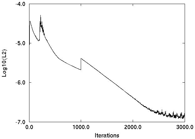
Figure 2. Plot of the L2 residual history.
The CFPOST utility was used to generate the data files for the boundary layer profiles at the end of the plate and skin-friction distribution along the plate.
cfpost < cfpost.bl.com
cfpost < cfpost.cf.com
The file cfpost.bl.com is a command file which writes out the x and y coordinates, u-velocity, v-velocity, and temperature at the end of the plate to the file bl.gen. This file is then processed by the Fortran program fppost1.f, which converts the boundary layer profiles into units of the similarity variables. The program outputs the files u.d and v.d containing the u and v velocity profiles in similarity coordinates. The results are are for "eta" values up to approximately 6.0.
The file cfpost.cf.com is a command file which writes out the x and y coordinates, u-velocity, and v-velocity along the plate to the file cf.gen. This file is then processed by the Fortran program fppost2.f, which computes the skin friction coefficient along the plate starting at the first point past the leading edge. The file cf.d is output by this program.
The Plot3d solution file fplam.q.dat can be created by CFPOST. The file is unformatted, single-block, and three-dimensional.
cfpost < cfpost.plot3d.com
The u and v velocity profiles at the end of the plate are compared to the Blasius solution in Figs. 3 and 4, respectively. The skin friction coefficients along plate is compared to the Blasius solution in Fig. 5. The comparisons are very good.
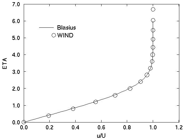
Figure 3. Comparison of the u-velocity at the end of the flat plate.
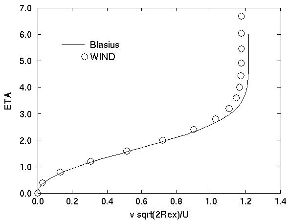
Figure 4. Comparison of the v-velocity at the end of the flat plate.
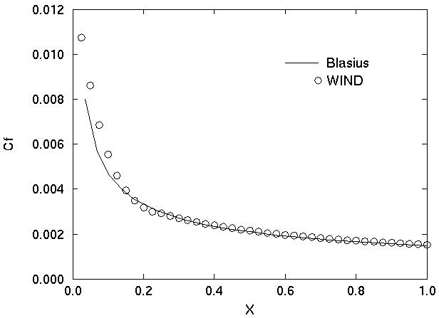
Figure 5. Comparison of the skin friction along the flat plate.
The computation of this case required 269.47 CPU seconds to run 3000 iterations with 6 cycles.
This case was created on April 30, 1998 and updated on July 14, 1999 by John W. Slater, who may be contacted at:
NASA John H. Glenn Research Center, MS 86-7
21000 Brookpark Road
Cleveland, Ohio 44111
Phone: (216) 433-8513
e-mail: John.W.Slater@grc.nasa.gov