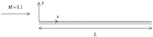
Figure 1. Geometric configuration for laminar flow past a flat plate.
Figure 1. Geometric configuration for laminar flow past a
flat plate.
This validation case involves the flow past a flat plate at zero angle of incidence. The Mach number of the flow is Mach 0.1, which can be assumed "incompressible". A laminar boundary layer develops on the plate and thickens along the plate.
| Mach | Pressure (psia) | Temperature (R) | Angle-of-Attack (deg) | Angle-of-Sideslip (deg) |
|---|---|---|---|---|
| 0.1 | 6.0 | 700.0 | 0.0 | 0.0 |
These conditions were chosen so that the Reynolds number based on the length of the plate (1.0 ft) was approximately 200000.
The flat plate has a length of 1.0 ft. The leading edge is located at x = 0.0 ft.
At the flat plate surface the no-slip condition applies. The inflow boundary of the computational domain is a subsonic inflow boundary and is placed upstream of the leading edge at x = - 0.25 ft so as to capture the leading edge flow. The outflow boundary is placed at the end of the plate at x = 1.0 ft. The farfield flow beyond the boundary layer should remain fairly uniform at freestream conditions. The farfield boundary is placed at about eta = 50.
The classical Blasius similarity solution provides data for comparison. The text by White discusses this solution.
The Fortran program blasius.f creates the following data files for comparison. The solution for the similarity equation is given in the file fplam.blasius. The data files are u.blasius, v.blasius, and cf.blasius.
The computational grid was generated by the Fortran program fpgrid.f. The grid points are evenly spaced along the plate according to the streamwise grid spacing specified. The normal grid points are placed at constant "eta" coordinates with the grid evenly spaced until "eta" = 4.0 and then spaced by a factor of 1.1 until the outer boundary at "eta" = 50 is reached. Thus, the number of streamwise and normal grid points are determined according to the desired spacings. Fig. 2 below shows how the grid looks.
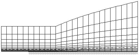
Figure 2. Computational Grid (coarsened for display).
| Study | Category | Person | Comments |
|---|---|---|---|
| Study #1 | Example | J. Slater | Single run |
White, F.M., Viscous Fluid Flow , McGraw Hill Inc., New York, 1974.
Questions or comments about this case can be sent be emailed John W. Slater at the NASA John H. Glenn Research Center.