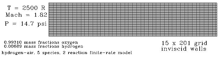
Figure 1: Schematic of Channel.
Figure 1: Schematic of Channel.
This study focuses on a finite-rate, hydrogen-oxygen chemical reaction occuring within a constant-area channel. The ignition point and species mass fraction values of the combustion products are investigated. The WIND (version 5.116 ALPHA) results are compared to Channel Combustion Study #1 (8-reaction model vs 2-reaction model shown here). All calculations presented here use a two-dimensional grid.
A 201 x 15 single-zone mesh was generated to model the channel region from 0 to 5 inches downstream. The channel is 5 inches long and 1 inch tall. The reference paper indicates that 201 points axially was adequate to predict the correct ignition point, based on a closed-form solution using rate equations.
This grid is provided below in Plot3d (two-dimensional, multiple-grid, unformatted, whole) and common file format. The coordinates in both files are in units of inches
| Plot3D | Common Grid |
| channel2.xyz | channel2.cgd |
The initial (freestream) conditions were set to static conditions of 2500 Rankine, a pressure of 14.7 psi, and Mach number 1.82. In addition, species mass fractions were set to 0.99310 for oxygen and 0.00689 for hydrogen (all others set to zero). The Fuel-to-Air ratio was set initially to 1, and then set to 2 in the middle of the calculation. No affect was seen on the solution (So the fuel to air ratio does nothing?). O2 and H2 mass fractions at the inflow plane remained at the initial values specified. In this case, the chemistry file h2air-5sp-std-15k.chm was used for the finite-rate calculations. The crossflow CFL and TVD factors were set to a value of 1. The flow in this case was considered laminar. The 2 reactions taking place are not present in the .chm file (i.e., they are unknown).
The frozen boundary condition was used for the inflow, inviscid or wall slip BC employed for the upper and lower walls, and the outflow boundary condition was used at the exit (forcing extrapolation of the pressure).
The computation is performed using the time-marching capabilities of WIND to march to a steady-state (time asymptotic) solution. Local time stepping is used at each iteration. The time-marching is performed until the convergence criteria is achieved. The solution ran for 6338 iterations at a CFL number of 0.05.
The input data file for WIND is channel2.dat.
The WIND flow solver is run, creating the following output files:
| Plot3D | Common File Solution | List File |
|---|---|---|
| channel2.q | channel2.cfl | channel2.lis |
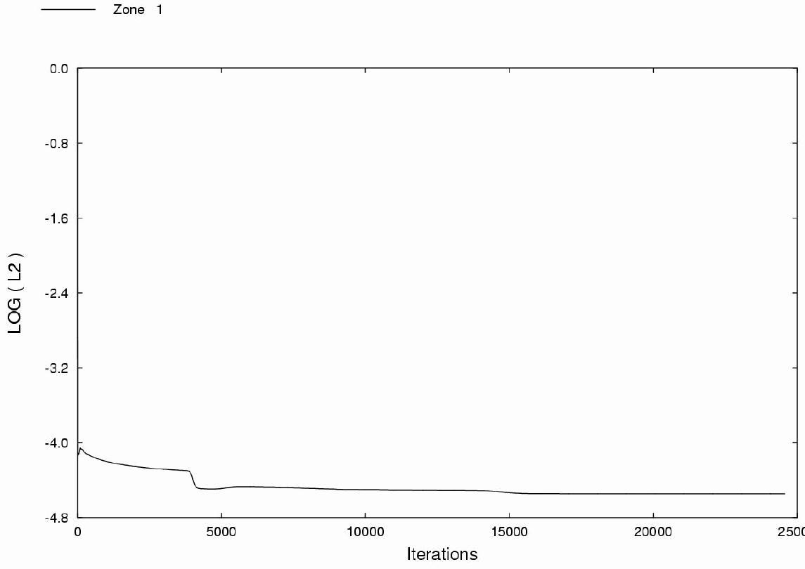
Figure 2: Plot of L2 Norm: Convergence history
Convergence information can also be obtained from the channel.lis file by using the resplt utility program.
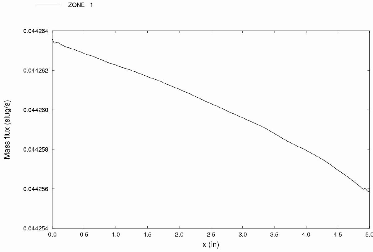
Figure 3: Mass flow
Species mass fractions for H2O, H2, and O2 can be compared to Channel Combustion Study #1. For Channel Study #2, The ignition point was found to occur immediately at the duct entrance. For Channel Study #1, the ignition point was found to occur about 0.78 inches downstream.
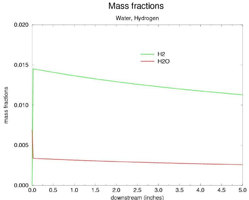
Figure 4: H2O and H2 mass fractions at duct centerline
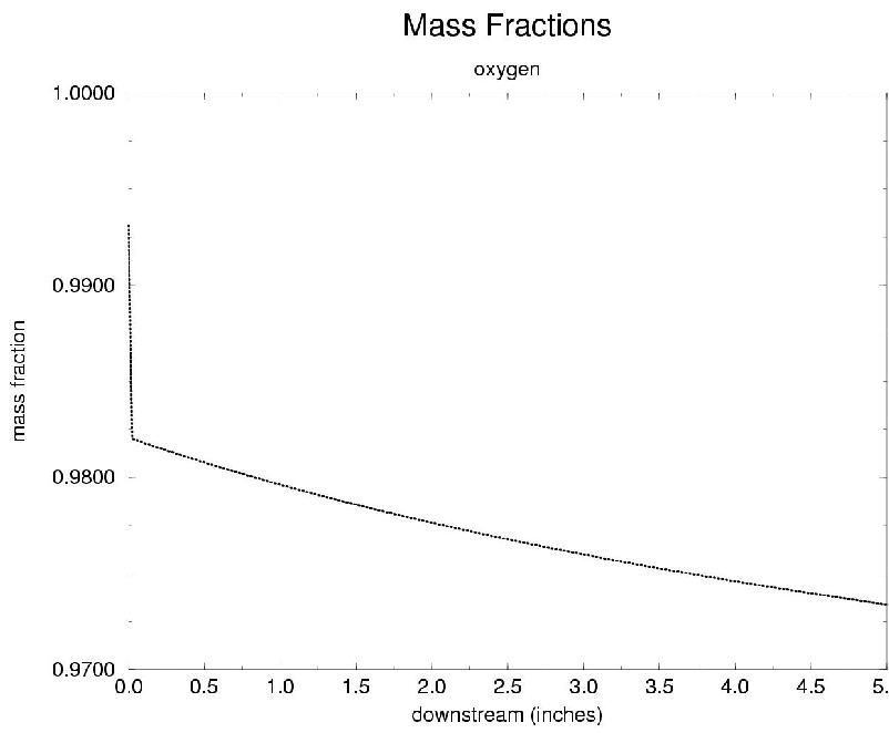
Figure 5: Oxygen mass fractions at duct centerline
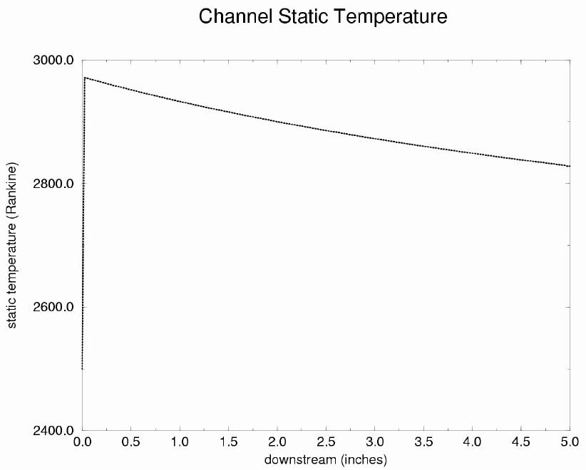
Figure 7: Static Temperature plot downstream at duct centerline
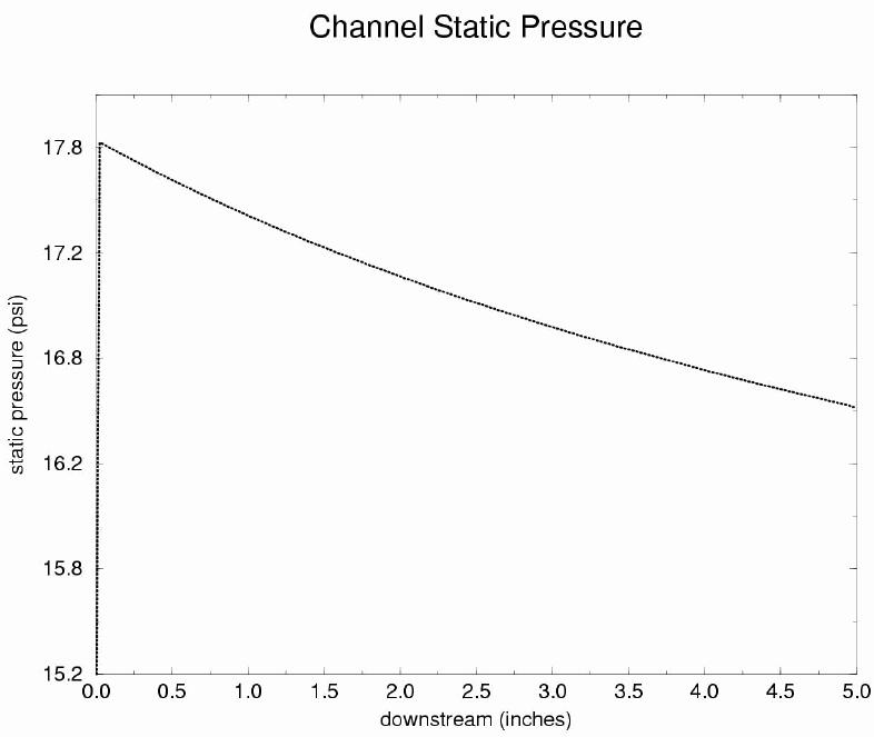
Figure 8: Static Pressure plot downstream at duct centerline
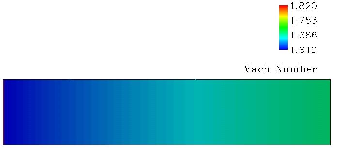
Figure 9: Mach Number contours in the x-y plane.
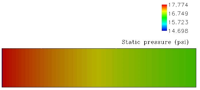
Figure 10: Static pressure contours in the x-y plane.
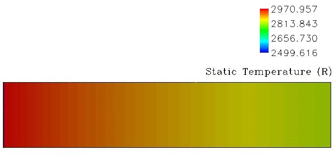
Figure 11: Static Temperature contours in the x-y plane.
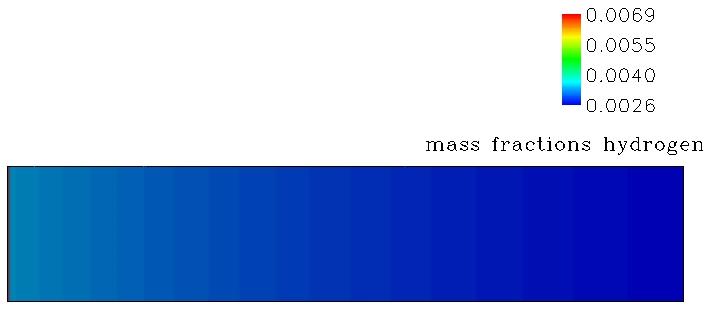
Figure 12: Hydrogen mass fractions contours in the x-y plane.
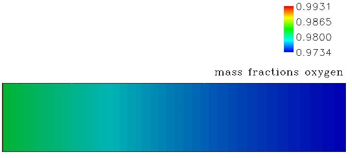
Figure 13: Oxygen mass fractions contours in the x-y plane.
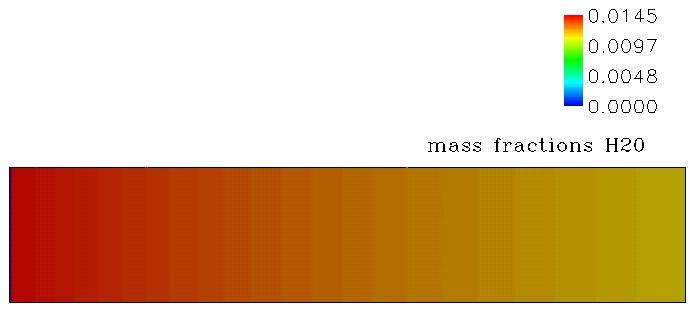
Figure 14: H2O mass fractions contours in the x-y plane.
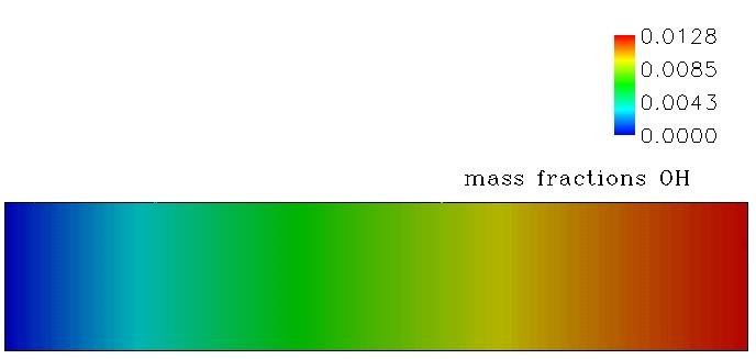
Figure 15: OH mass fractions contours in the x-y plane.
Mani, M., Bush, R.H., Vogel, P.G., "Implicit Equilibrium and Finite-Rate Chemistry Models For High Speed Flow Applications," AIAA Paper 91-3299-CP, Jan. 1991.
This case was created on March 5, 2002 by Teryn DalBello, who may be contacted at
NASA Glenn Research Center, MS 86-7
21000 Brookpark Road
Cleveland, Ohio 44111
Phone: (216) 433-8412
e-mail: teryn@grc.nasa.gov