
The Modular Aerodynamic Design Computational Analysis Process (MADCAP) "Create" library and menus are used to create new objects such as points, curves, surfaces, and zones. Typically, objects created using this menu are made "from scratch", whereas objects created by using the Manipulate Menu are composed of portions of the object from which they are derived.
Selection of the "Create" menu item produces the drop down menu shown below.
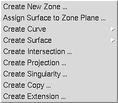
There are ten selections under the Create menu. They are:
Help on these submenus is available below.
Selection of the "Create New Zone ..." submenu causes the following window to be displayed.
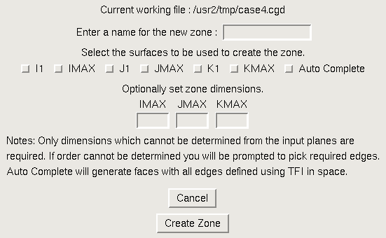
This operation simply creates a new zone and defines its name and dimensions. If the working file is a .cgd file, the zone will be created of the specified size, and all points in the zone will be at (0.,0.,0.). More typically, this operation is used when the working file is a .csf file, to define a new, empty zone whose faces will be assigned as they are created using other program functions (see the Assign Surface to Zone Plane menu item).
To create a new zone definition, the user simply needs to enter a name and dimensions for each of the three computational directions in the appropriate entry boxes, and then click the "Create Zone" button. To escape from this window with no action being taken, select the "Cancel" button.
The text commands generated by this operation are:
   create zone imax imax jmax jmax kmax kmax
   file save name zonename
Selection of the "Assign Surface to Zone Plane ..." submenu causes the following window to be displayed.
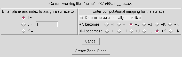
This operation is used to assign a surface generated in MADCAP a definition in an existing zone. For example, through several other MADCAP create, manipulate, or grid generation operations, the user may have generated a surface to serve as the J = 1 boundary of an existing zone. (If no zone exists for the boundary yet, it must be generated first using the Create Zone operation first). To make the assignment, this operation is used. The user would set the radiobutton to the left of the window to J, and ensure that a 1 is entered in the entry box for the J index being assigned. The user must also specify a mapping to transform the N, M computational indices of the surface to the appropriate I, J, and K computational indices of the zone. The Highlight Object Origins option under the view menu is often helpful in making this determination. Once a single zone face exists in a zone, it is often possible for MADCAP to automatically determine the correct transformation for adjacent faces by comparing edges of the surfaces. If the user would like the program to determine the transformation, simply select the checkbutton on the right.
Selecting the "Create Zone Plane" button will cause the main program to prompt first for a surface to assign to a zone, and then for the zone the surface is to be assigned to. MADCAP will then create a new zone plane in the specified zone. If any edge mismatches occur where the new zone plane abuts existing zone planes, an error message is generated indicating the magnitude of the mismatch relative to local grid spacings. Small mismatches can usually be ignored, but larger mismatches should usually be investigated to determine the source of the problem. In any event, the zone plane is created even if mismatches exist along edges.
To escape from this window with no action being taken, select the "Cancel" button.
The associated text command is:
   create zplane {i | j | k} index nmap {auto | +i | -i | +j | -j | +k | -k} \
      [mmap {+i | -i | +j | -j | +k | -k }]
Selection of the "Create Curve" submenu causes the cascade menu shown below to be displayed.
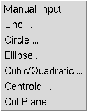
Seven different methods are provided for creating independent curves from scratch. These methods are:
Help on these submenus is available below.
Selection of the "Manual Input ..." submenu causes the following window to be displayed.
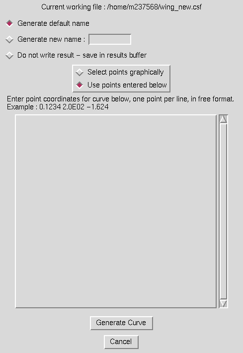
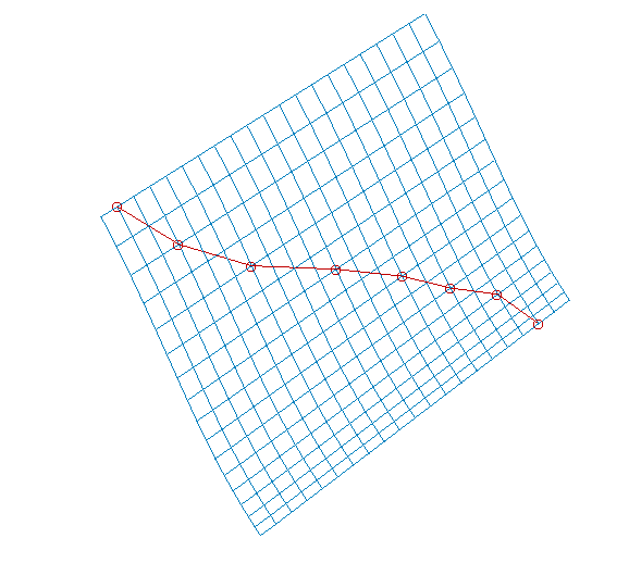
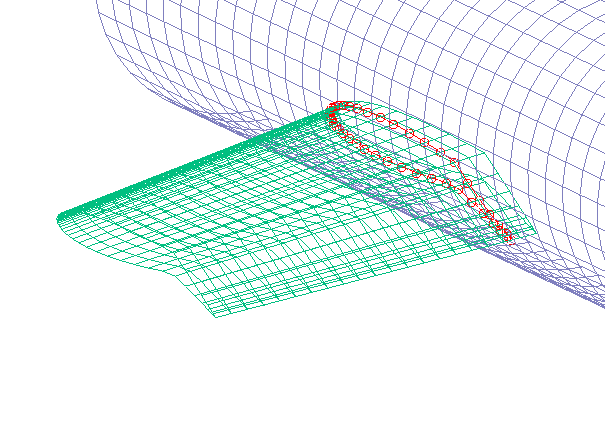
This operation is used to create a curve completely from scratch. The individual points making up the curve can either be input graphically from the screen or by typing in the coordinates desired in the large entry box in the window. The radiobutton must be set to match the style of input desired. If points are typed in at this window, they should be entered in free format, one point per line. Note also that the standard X-windows cut and paste utilities can be used to insert a multi-lined file in this format into the window. The user should also select the appropriate radiobutton at the top of the screen to have the program either generate a default name, use a specified new name, or simply save the result in the object manager results buffer. Finally, the user should select the "Generate Curve" button. If the points are to be entered graphically, the program will prompt for points to make up the curve until the "done" button on the main graphics screen is selected. The red curve in the image below is an example of a manual-input curve defined by graphically selecting specific points from the larger surface to generate a new curve.
The text commands generated are:
   om select point point_definition (Multiple instances)
   create manual_curve
   file save {default | name curvename}
Selection of the "Line ..." submenu causes the following window to be displayed.
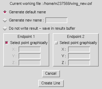
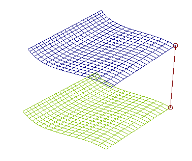
This operation is used to create a curve consisting of simply a straight line between two endpoints. The endpoints may either be selected graphically by setting the checkbuttons in the window, or the x, y, and z values for the endpoints may be set in the entry boxes. Radiobuttons should also be set to generate either a default name, a specified name, or to save the line in the object manager results buffer. When the "Create Line" button is selected, the program creates the line or prompts for inputs first if the endpoints are being selected graphically. The red line in the image below is an example of a line generated by graphically selecting the corner points of two displayed surfaces.
The text commands generated are:
   om select point point_definition (Two instances)
   create line curve
   file save {default | name curvename}
Selection of the "Circle ..." submenu causes the following window to be displayed.
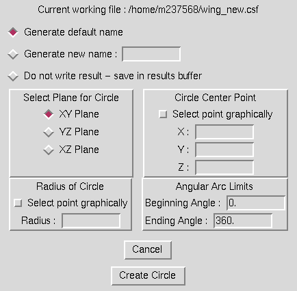
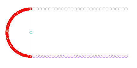
This operation is used to create a curve consisting of a circular arc. Circular arcs can be generated parallel to the xy plane, yz plane, or xz plane by selecting the appropriate radiobutton. A center for the circle must be defined either by entering coordinates in the entry boxes or having the program prompt to select the center from the graphical display. Similarly, the radius may be entered in the entry box or a point may be picked from the graphics screen which will define the radius relative to the centerpoint. Finally, the portion of the defined circle to be generated is defined by setting the angular arc limits between 0 and 360 degrees. Radiobuttons should also be set to generate either a default name, a specified name, or to save the line in the object manager results buffer. When the "Create Circle" button is selected, the program will either prompt for graphical selections or generate the defined circular arc. A point is generated every 1 degree of the circular arc. The red curve in the image below is an example of a circular arc defined with the center at the midpoint of the first end of the two lines and a radius defined by selecting the first endpoint of one of the lines. The beginning and ending arc values are defined in a standard right-handed sense. For the circle below in the yz plane, the angle limits entered were 90 and 270 degrees.
The text commands generated are:
   om select point point_definition (One instance, to define center)
   om select point point_definition (One instance, if defining radius
      graphically)
   create circle plane {xy | xz | yz} [radius radius] start angle end angle
   file save {default | name curvename}
Selection of the "Ellipse ..." submenu causes the following window to be displayed.
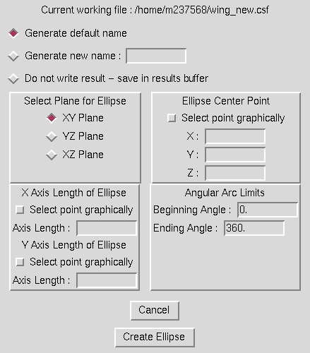
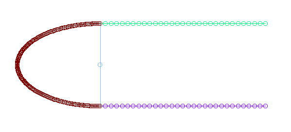
This operation is used to create a curve consisting of an elliptical arc. Elliptical arcs can be generated parallel to the xy plane, yz plane, or xz plane by selecting the appropriate radiobutton. A center for the ellipse must be defined either by entering coordinates in the entry boxes or having the program prompt to select the center from the graphical display. Similarly, the two axis lengths may be entered in the entry box or points may be picked from the graphics screen which will define the axes relative to the centerpoint. Finally, the portion of the defined ellipse to be generated is defined by setting the angular arc limits between 0 and 360 degrees. Radiobuttons should also be set to generate either a default name, a specified name, or to save the line in the object manager results buffer. When the "Create Ellipse" button is selected, the program will either prompt for graphical selections or generate the defined elliptical arc. A point will be generated every 1 degree on the elliptical arc. The red curve in the image below is an example of an elliptical arc defined with the center at the midpoint of the first end of the two lines, one axis defined by selecting the first endpoint of one of the lines, and the other axis defined by a keyed in length. The beginning and ending arc values are defined in a standard right-handed sense. For the ellipse below in the yz plane, the angle limits entered were 90 and 270 degrees.
The text commands generated are:
   om select point point_definition (One instance, to define center)
   om select point point_definition (Additional instances, if defining
      axes graphically)
   create ellipse plane {xy | xz | yz} [aaxis aaxis] [baxis baxis] \
      start angle end angle
   file save {default | name curvename}
Selection of the "Cubic/Quadratic ..." submenu causes the following window to be displayed.
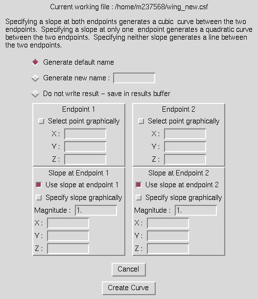
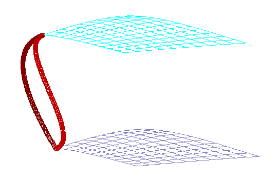
This operation is used to create either cubic or quadratic curves. The user must define the two endpoints for the curve, either by selecting the checkbutton to select them graphically or by entering coordinates in the entry boxes. To define a cubic curve, the checkbuttons to use the slope information at both endponts should be selected. For a quadratic curve, slope information is included at only one of the endpoints. Slopes may also be defined either graphically or by entering the components of the slope vector relative to (0,0,0) in the entry boxes. If slopes are defined graphically, the user is prompted for two points which define the slope vector direction. The magnitude entry boxes must be filled out for the ends where slope is being defined. This value controls the shape of the curve. Higher values cause the slope direction to be maintained for longer arc length of the final curve than lower values. Radiobuttons should also be set to generate either a default name, a specified name, or to save the line in the object manager results buffer. When the "Create Curve" button is selected, the program will either prompt for graphical selections or generate the defined cubic or quadratic. The red curves in the image below are examples of cubic and quadratic curves generated between two surface points. For each curve, the slope was controlled at the top to match the slope of the surface, but the slope at the bottom was only controlled on the cubic curve. Note that if slope is controlled at neither end, the operation defaults to generating a line between the two endpoints, just as if the Create Line menu option had been selected.
The text commands generated are:
   om select point point_definition (Two instances, to define endpoints)
   om select point point_definition (Two instances per slope, if defining
      slopes graphically)
then
   create cubic curve [slope1 x y z ] [slope2 x y z ] first_mag magnitude \
      last_mag magnitude
or
   create quadratic curve slope_end {first | last} [slope x y z ] \
      magnitude magnitude
or
create line curveand finally
file save {default | name curvename}
Selection of the "Centroid ..." submenu causes the following window to be displayed.
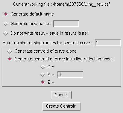
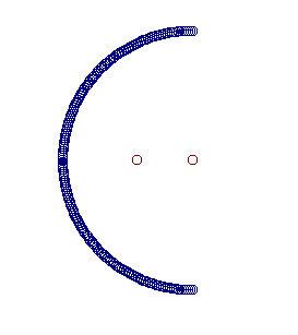
This operation is used to generate the centroid of a curve. Optionally, the user can generate a singularity at the centroid by specifying how many times to duplicate the point generated as the centroid. Also, the user may generate the true centroid of the curve, or the centroid of the curve including its reflection about any plane perpendicular to a principal plane. This is especially useful when working with only one half of a symmetric geometry. In this case, the radiobutton for which type of symmetry plane is being used must be set, as well as a value for the location of the plane. Radiobuttons should also be set to generate either a default name, a specified name, or to save the centroid in the object manager results buffer. When the "Create Centroid" button is hit, the program will prompt for the curve to generate a centroid for. The two red points in the image below show the results of generating a centroid for the circular arc with and without using the reflection option.
The text commands generated are:
   om select curve curve_definition
   create centroid curve nsing n_singularities [refplane {x | y | z} value]
   file save {default | name curvename}
Selection of the "Cut Plane ..." submenu causes the following window to be displayed.
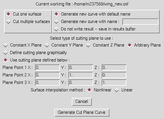
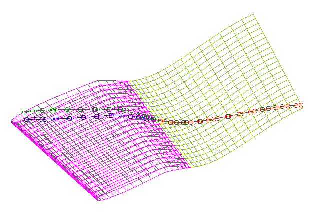
This operation is used to generate a curve by passing a cutting plane through a surface or set of surfaces. The user should first indicate whether to cut a single surface or multiple surfaces using the radiobuttons at the top left of the window. The type of plane to be used for cutting should then be set to either a constant x, y, or z plane, or an arbitrary plane. Only a single point is required to define the cutting plane for the first three options, while three points are required to define an arbitrary plane. The user may choose to define the point or points defining the cutting plane graphically or by entering coordinates in the entry boxes shown. The user must also specify whether to use linear or nonlinear interpolation when cutting through the cells defining the surface being cut. Each surface cut generates a separate curve, and if a cut through a surface generates multiple curves, each curve is output individually. Radiobuttons should also be set to generate either a default name, a specified name, or to save the centroid in the object manager results buffer. When the "Create Cut Plane Curve" button is selected, the program prompts for the surfaces to be cut, and the point(s) defining the plane if they are to be entered graphically. The red and blue curves in the image below show an example of a cutting plane through multiple surfaces.
The text commands generated are:
   om select surface surface_definition (Multiple instances, to define
      surfaces being cut)
   om select point point_definition (One or three instances, to define
      cutting plane)
   create cutplane {x | y | z | arb} interp {linear | nonlinear}
   file save {default | name curvename}
Selection of the "Create Surface" submenu causes the cascade menu shown below to be displayed.
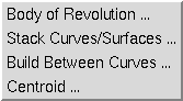
Four different methods are provided for creating surfaces entirely from scratch. These methods are:
Help on these submenus is available below.
Selection of the "Body of Revolution ..." submenu causes the following window to be displayed.
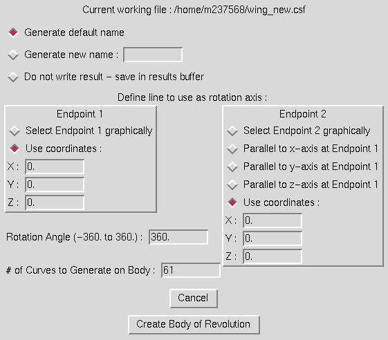
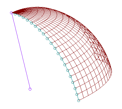
This operation is used to generate a surface by rotating a curve about a line an input angular distance and saving the surface thus swept out. The user must set the radiobutton for the first endpoint of the line to rotate about to either identify the endpoint graphically or use the coordinates entered into the entry boxes. To define the rotation line, the user can then specify that the line is simply parallel to either the x, y, or z axes at the first endpoint, or may again select an endpoint graphically or by using the entry boxes. The rotation angle (0 to 360 degrees) must then be entered, as well as the number of curves to generate on the resulting surface. The curve being rotated will become the N = 1 line on the surface, and Nmax will be the number entered here. (Mmax will remain the number of points on the curve being rotated.) Radiobuttons should also be set to generate either a default name, a specified name, or to save the body of revolution in the object manager results buffer. When the "Create Body of Revolution" button is selected, the program prompts for the curve to be rotated, and the point(s) defining the rotation line if they are to be entered graphically. The red surface in the image below shows an example of a body of revolution generated by rotating the blue curve 90 degrees about the purple line.
The text commands generated are:
   om select curve curve_definition (One instance, to define curve to
      rotate)
   om select point point_definition (One or two instances, to define line
      to rotate about)
   create body_of_rev parallel_to {line | x | y | z} angle value \
      ncrvs value
   file save {default | name surfacename}
Selection of the "Stack Curves/Surfaces ..." submenu causes the following window to be displayed.
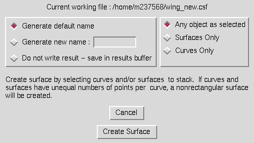
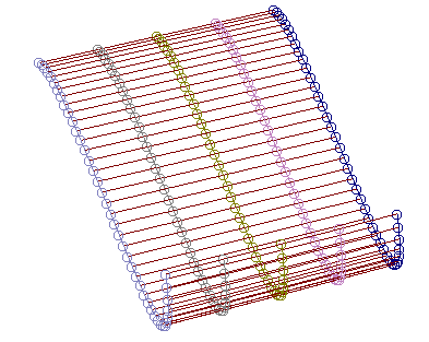
This operation is used to generate a surface by simply stacking several independent curves as constant N-lines to create a new surface. Thus, the order of points on the curves selected as well as the order in which these curves are selected are both critical in determining the definitions of the new surface generated. Since surfaces can be viewed as simply a collection of previously stacked curves, it is even possible to include surfaces in the select buffer. In this case, the individual N-lines from the surface are stacked in the new surface just as if they had each been selected individually. The user needs only to specify whether the program should interpret picks on surfaces as selecting the specific curve picked on or as selecting the entire surface for inclusion in the final surface. The user should also set the radiobuttons at the upper left to define whether to generate a default name, a specified name, or to save the new surface in the object manager results buffer. When the Create Surface" button is selected, the program prompts for the curves and or surfaces to be stacked to generate the new surface. The red surface in the image below shows an example of a surface generated by stacking the individual displayed curves. Note that in this image, the N-lines on the resulting surface are obscured by overplotting the individual curves stacked to create the surface to show how the operation works. Without these curves displayed, the N-lines on the resultant surface would also be drawn in red.
The text commands generated are:
om select curve curve_definition (Multiple instances)and/or
om select surface surface_definition (Multiple instances)followed by
   create stack
   file save {default | name surfacename}
Selection of the "Build Between Curves ..." submenu causes the following window to be displayed.
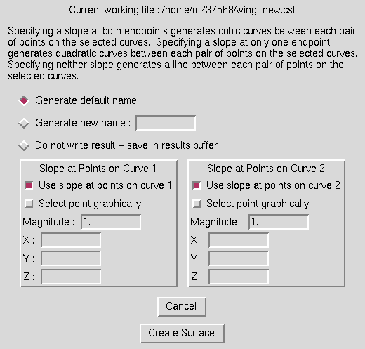
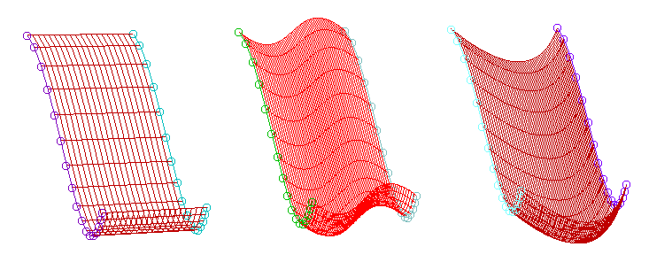
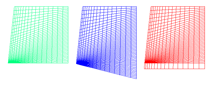
This operation is used to generate a surface between two curves containing the same number of points. The surface generated can consist of straight lines, cubic curves, or quadratic curves between pairs of curve points. To generate straight lines, set the checkbuttons to use the slope at neither of the two curves being built between. For a cubic, slopes must defined at both curves, and for a quadratic, at either one of the curves. Slopes can be defined either graphically or by entering the components of the slope vector relative to (0,0,0) in the entry boxes. If slopes are defined graphically, the user is prompted for two points which define the slope vector direction. The magnitude entry boxes must be filled out for the curves where slope is being defined. This value controls the shape of the final surface. Higher values cause the slope direction to be maintained for a longer arc length of the final surface than lower values. Radiobuttons should also be set to generate either a default name, a specified name, or to save the surface in the object manager results buffer. When the "Create Surface" button is selected, the user will be prompted for the two curves to be built between as well as any points to define slopes graphically. The red surfaces in the images below are examples of building linear, cubic, and quadratic surfaces between the end curves.
The text commands generated are:
   om select curve curve_definition (Two instances, to define curves to
      build between)
   om select point point_definition (Two instances per slope, if defining
      slopes graphically)
followed by
   create cubic surface [slope1 x y z] [slope2 x y z] first_mag magnitude \
      last_mag magnitude
or
   create quadratic surface slope_end {first | last} [slope x y z ] \
      magnitude magnitude
or
create line surfaceand finally
file save {default | name curvename}
Selection of the "Centroid ..." submenu causes the following window to be displayed.
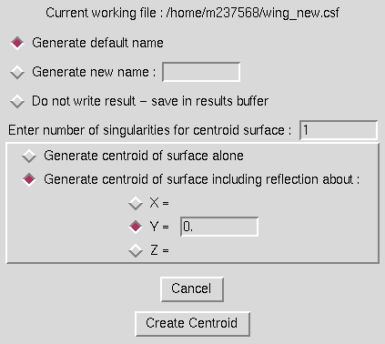
This operation is used to generate a curve or a singular surface composed of the centroids of the constant N-lines on a surface. Optionally, the user can generate a singular surface by specifying how many times to duplicate the curve generated at the curve centroids. Also, the user may generate the true centroids of the N-lines, or the centroids of the N-lines including the reflection about any plane perpindicular to a principal plane. This is especially useful when working with only one half of a symmetric geometry. In this case, the radiobutton for which type of symmetry plane is being used must be set, as well as a value for the location of the plane. Radiobuttons should also be set to generate either a default name, a specified name, or to save the centroid in the object manager results buffer. When the "Create Centroid" button is hit, the program will prompt for the surface to generate a centroid for. The blue and red curves in the image below show the results of generating a centroid for the surface with and without using the reflection option.
The text commands generated are:
   om select surface surface_definition
   create centroid surface nsing n_singularities [refplane {x | y | z} value]
   file save {default | name curvename}
Selection of the "Create Intersection ..." submenu causes the following window to be displayed.
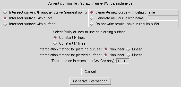
This operation is used to generate a curve by the intersection of two surfaces or the intersection of a surface with a family of curves on a surface, or to create a point by the intersection of two curves. The intersection mode is set by selecting the corresponding radio button at the top left of the window.
If the intersection of two curves is selected, the user may specify a tolerance for this intersection in the text field at the bottom of the window.
If surface-surface intersection is selected, the user must set which family of lines to use to create the intersection. Both these piercing curves and the intersected, or pierced, surface can be interpolated on using linear or nonlinear interpolation as set with the radiobuttons at the bottom of the window.
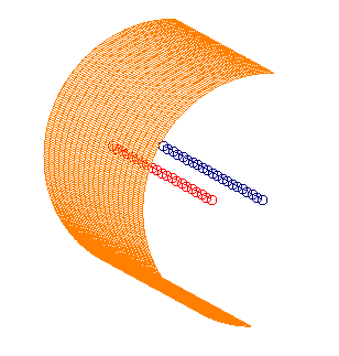
Note that for surface-surface intersections, it is possible to get four different definitions of the intersection curve, depending on which surface is used as the piercing surface and the family of grid lines used to pierce with. (Pierce with N-lines on surface 1, M-lines on surface 1, N-lines on surface 2, or M-lines on surface 2.) It is typically best to select whichever family of curves would result in the best definition of an intersection for the piercing curve. Radiobuttons should also be set to generate either a default name, a specified name, or to save the new curve in the object manager results buffer. When the "Create Intersection" button is hit, the program will prompt for the two objects to intersect. The red curve in the image below shows the result of intersecting the other two displayed surfaces.
The text commands generated are:
om select surface surface_definition (Two instances)or
   om select curve curve_definition
   om select surface surface_definition
followed by
   create intersection linetype {n | m} interp1 {linear | nonlinear} \
      interp2 {linear | nonlinear}
   file save {default | name curvename}
Selection of the "Create Projection ..." menu causes the following window to be displayed.
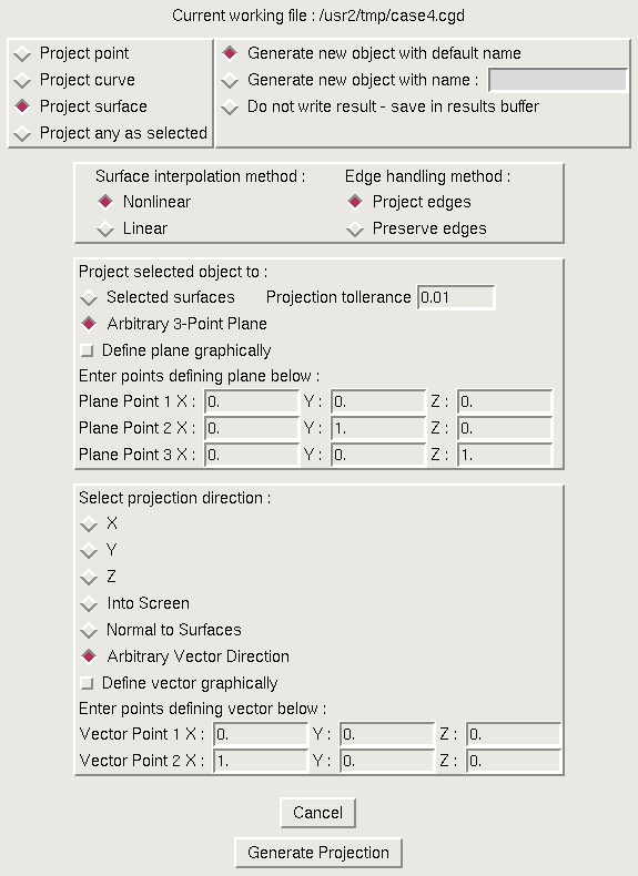
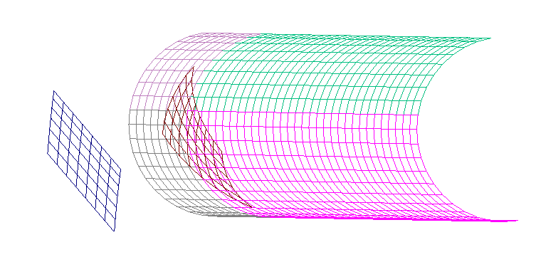
This operation is used to generate the projection of an object to a plane or a set of existing surfaces. For projection to surfaces, the user must first define how to interpolate on the surfaces, linear or nonlinear. Since often it is desirable to project only the interior points of a surface and leave the edges untouched, radiobuttons are also provided to allow this. In the middle of the window, the user sets whether to project to a plane or a set of surfaces. If projecting to a plane, it may be defined graphically by picking three points on the display, or the coordinates may be entered in the entry boxes. The last area of the window controls the direction for the projection. The projection can be made in the x, y, or z directions or in an arbitrary direction. Arbitrary directions can be defined by specifying a direction into the current graphics screen, by selecting two points on the screen to define a vector, or by entering coordinates defining a vector direction into the window entry boxes. Projection can also be made normal to the surfaces projecting to (that is, to the closest point on the set of surfaces projecting to). Radiobutton should also be set to generate either a default name, a specified name, or to save the new curve in the object manager results buffer. When the "Create Projection" button is hit, the program will prompt for the object to project, as well as the points defining a plane and the vector direction if these options are set. The red surface in the image below shows the result of projecting the blue surface to the other displayed surfaces.
The text commands generated are:
   om select objecttype object_definition
   om select point point_definition (Multiple instances, to define
      projection plane)
   om select point point_definition (Multiple instances, to define
      projection direction)
   create project to {plane | surfaces} direction {x | y | z | normal | \
      arb} interp {linear | nonlinear} edges {projected | original}
   file save {default | name objectname}
Selection of the "Create Singularity ..." submenu causes the window below to be displayed.
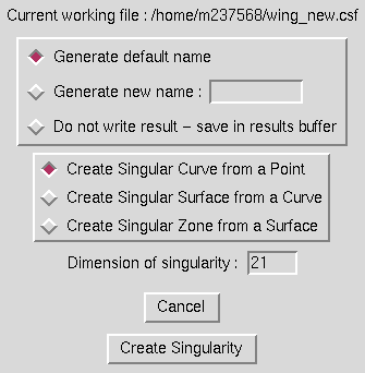
This operation is used to generate a singular object one order higher than the selecting object by duplicating its definition an input number of times and making that number the next higher dimension. Thus, a singular curve can be made by duplicating a point, a singular surface can be made by duplicating a curve, and a singular zone can be made by duplicating a surface. The user simply needs to specify which type of singularity is being created, and enter a dimension for the singularity. Radiobuttons should also be set to generate either a default name, a specified name, or to save the new object in the object manager results buffer. When the "Create Singularity" button is hit, the program will prompt for the object to be duplicated. Since no change in the display is noticeable for this operation, no example is shown.
The text commands generated are:
   om select objecttype object_definition
   create singularity dimension n_duplications
   file save {default | name objectname}
Selection of the "Create Copy ..." submenu causes the window below to be displayed.
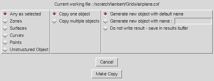
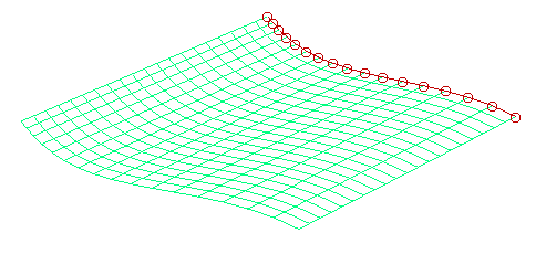
This option is used to create a copy of an entity. By selecting a curve from a surface and issuing a copy command, the user can extract a curve off a surface and save it as an independent object. Similarly, a point could be extracted from a curve or a surface from a zone in this manner. Although not currently possible from the GUI, in text mode the copy command can also be used to extract a subregion of an object of the same dimension to save as an independent object - that is, extract only points 5 through 10 from a curve with 20 points on it. From the GUI window, the user needs only to specify the types of objects to copy, whether to prompt for multiple objects, and specify whether to generate a default name, a specified name, or to save the new object in the object manager results buffer. When the "Make Copy" button is hit, the program prompts for the objects to be copied and generates the copies. In the image below, the red curve was copied off of the surface and saved as an independent object.
The text commands generated are:
   om select object_type object_definition (Multiple instances)
   create copy
   file save name objectname
Selection of the "Unstructured Object" radio button causes the window to display further options for creating copies of unstructured objects, as shown in the following example.
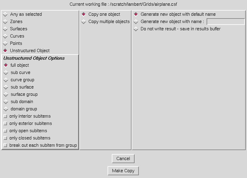
A list of unstructured sub-entities is displayed in the bottom left of the window. Here the user may select the type of sub-object to be copied out of the original unstructured object by selecting one of the radio-button boxes (diamond shape boxes). Possible selections are to copy out a sub-curve, sub-curve group, sub-surface, sub-surface group, sub-domain, or sub-domain group. In addition, the user may further restrict which items should be selected by selecting one or more modifier check boxes (square boxes). The modifiers include interior subitems, exterior subitems, open subitems, and closed subitems. Interior subitems are items that are on the interior of an object. For instance, an interior sub-curve lies on the interior of a surface mesh (not on the outer loop). An open subitem is a non-closed item. For instance, an open curve would have differing first and last points, whereas a closed curve would contain the same first and last point (forms a closed loop).
All of the sub-surfaces of an object can be copied by selecting "full object" and selecting the "break out each subitem from group" boxes. All of the sub-surfaces of an surface group can be copied by selecting "surface group" and selecting the "break out each subitem from group" boxes.
Selection of the "Create Extension ..." submenu causes the following window to be displayed.
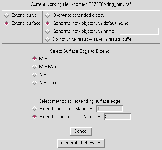
This option is used to either extend one end of a curve or to extend one of the four sides of a surface. The user must set the radiobutton at the upper left to indicate whether a curve or surface is to be extended. For a curve, the user must then set whether to extend the M = 1 or M = max end of the curve. For a surface, the N = 1 and N = max sides can also be extended. The curve or surface is then extended by adding points to the surface in the direction defined by the cell(s) at the end of the curve or surface. There are two methods for extending a surface or curve. First, the user can simply specify a constant distance to extend the end or side. Secondly, the user can have the program simply add a specified number of cells to the end or side. For this case, the cell size at the end is duplicated as many times as requested. The user must also specify whether to generate a default name, a specified name, or to save the new object in the object manager results buffer. When the "Generate Extension" button is hit, the program prompts for the object to be extended and generates the extended surface or curve. In the image below, the red surface shows a surface edge extended a constant distance, and the blue surface shows a surface edge extended by adding 11 cells to the green surface. (Surfaces translated to show differences. Otherwise new surfaces would totally obscure original surface which exists as a subset of the new surface.)
The text commands generated are:
   om select object_type object_definition
   create extend edge {m1 | mm | n1 | nm} {distance dist | ncells ncells}
   file save name zonename
Last updated 12 June 2007