
The Modular Aerodynamic Design Computational Analysis Process (MADCAP) "Grid Generation" library and menus are used to redistribute grid points on existing surfaces or run elliptic smoothing on existing grids.
Selection of the "Grid Generation" menu item produces the drop down menu shown below.
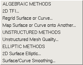
There are five selections under the Grid Generation menu. They are:
Help on these submenus is available below.
Selection of the "2D TFI ..." submenu causes the following window to be displayed.
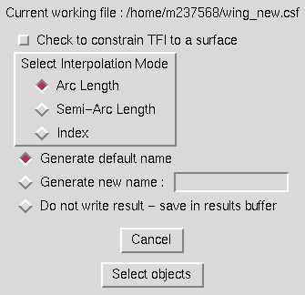
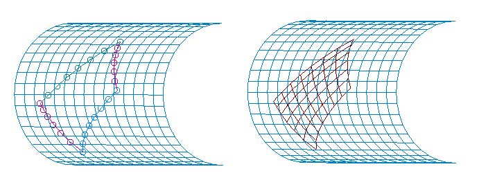
This is the window which is displayed if the checkbutton is not set to constrain the TFI to a structured grid surface. In this case, the user needs only to select the type of interpolation to use, and the program will prompt for four curves to generate a transfinite interpolation within. For this operation, opposite curves must have the same number of points, and the four curves must meet at the endpoints. An example of a surface generated by 2D TFI in space is shown below. The red surface was generated within the four curves. (The surface has been translated to avoid overplotting the four curves.)
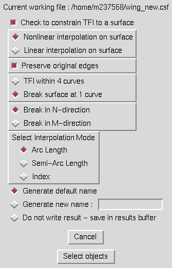
If the box is checked to constrain the TFI to a surface, the window is modified as shown below.
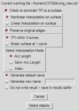
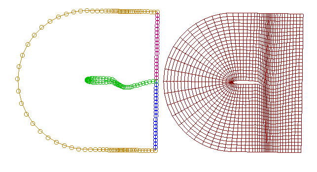
If the option is set to perform TFI within 4 curves, the user must select four curves which lie on the same surface, and the resultant surface will be constrained to lie on the structured grid surface as well. The user must additionally specify an interpolation mode on the structured grid surface (linear or non-linear) and whether to preserve the original edges or use a re-projected computation of the edges. An example of TFI on a structured grid surface is shown in the image below, where the red surface was generated within the four curves on the centerbody.
If the radiobutton is set to "Break Surface at 1 Curve", the window is modified as follows:
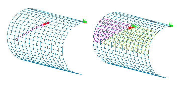
In this case, one additional input is required from the user - "Break in N- or M- direction". For this type of TFI on a surface, only a single curve lying on the surface is required. Two surfaces are generated from the curve, using either the N- or M- location of the endpoints as a constant and interpolating across the other direction to the surface's extremes. An example helps to clarify this process. In the following example, the surface was broken at the curve in the N-direction. New surfaces are extended out from the curve in the N direction to the N = 1 and N = max limits of the surface.
In the following image, the surface was broken at the curve in the M-direction. New surfaces are extended out from the curve in the M direction to the M = 1 and M = max limits of the surface.
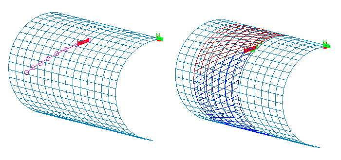
In both examples, the generated surface grids have the same number of points as the curve being broken at for the family of lines abutting that curve. The density of the surface grid being broken is used as a guide for generating the grid lines extending to the surface limits.
For any type of TFI, the user must also select a radiobutton to indicate whether to generate a default name, use a specified name, or save the result in the results buffer. When the "Select objects" button is selected, the program will prompt for either one or four curves, and for a surface if the TFI is to be constrained to a surface.
The text commands generated by this operation are:
   om select curve curve_definition (One or four instances)
   om select surface surface_definition (If constrained to a surface)
   ggs tfi 2d {space | surface} interp_mode {arc | semi | index} \
      [project {linear | nonlinear}] [edges {original | projected}] \
      [dir {n | m}]
   file save {default | name objectname]
Selection of the "Regrid Surface or Curve ..." submenu causes the following window to be displayed.
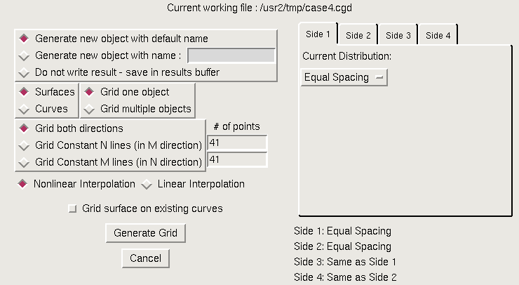
This operation is used to change the distribution of grid points on any surface or curve object.
For a surface, to do this in the most general sense the user selects the "Grid both directions" radio button, and specifies a new number of points for each direction (N and M), and a new point distribution function to apply on each of the four sides of the surface. The user can then enter the new number of points desired for both directions and select a distribution function for each of the four sides. The distribution function to be used for each side is determined by first selecting one of the four tabs (Side 1 through Side 4), then selecting the desired distribution from a dropdown menu opened by clicking the entry showing the current distribution. (More on distribution functions later.)
Optionally, the user may choose to only redistribute points on the surface in one direction, leaving the distribution of points in the other direction alone. To do this, the "Grid Constant N lines" or "Grid Constant M lines" radio button should be used, and only the side 1 and 3 distributions (for "Grid Constant N lines") or side 2 and 4 distributions (for "Grid Constant M lines") should be specified.
If the "Curves" radio button is used, rather than "Surfaces", only the Side 1 distribution function should be specified, since only a single distribution function is required for an isolated curve.
Multiple curves or surfaces may be gridded with the same regridding definition by selecting the "Grid multiple objects" radio button. The user must also specify whether to use nonlinear or linear interpolation when redistributing points.
As described above, the distribution function to be used for each side is chosen from a dropdown menu listing the available distributions. The dropdown menu for Side 1 is shown below.
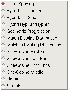
The various distribution functions are described in the following sections.
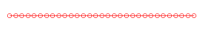
The equal spacing distribution function simply computes the arc length of the curve or surface edge and then distributes the requested number of grid points along the curve such that the distance from one point to the next remains constant. An example line with 31 points equally distributed is shown below.
The hyperbolic tangent distribution function is used to set a fixed cell size at one or both ends of the curve or edge, and distribute the remaining points such that the cell lengths grow or shrink by a hyperbolic tangent function. This function requires several additional inputs as shown in the window below. These buttons appear at the bottom of the list of distribution functions for any side whose option is set to "Hyperbolic Tangent".
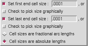
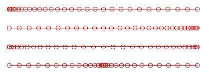
Depending on which checkbuttons are set, the user should enter the desired cell size for each end of the curve. These lengths may also be entered by picking a line segment graphically from the screen. If this mode of defining the cell lengths is chosen, the checkbuttons should be set and the program will prompt for the inputs at the appropriate time. If values are entered in the window, the user should use the final set of radiobuttons to indicate whether the numbers entered should be interpreted as absolute distance values for the length of the first cell or fractional values defining the size of the first cell relative to the total arc length of the curve or edge being regridded. The three curves below show the results of regridding a line with 31 points, with a cell size of .001 of the total arc length, applied at the first end, last end, and at both ends.
The hyperbolic sine distribution function is used to set a fixed cell size at a point on a curve or edge at either end or at an interior location on the curve or edge, and distribute the remaining points such that the cell lengths grow or shrink from this point by a hyperbolic sine function. This function requires several additional inputs as shown in the window below. These buttons appear at the bottom of the list of distribution functions for any side whose option is set to "Hyperbolic Sine".
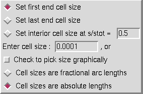
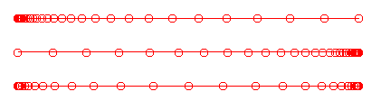
The user should set the desired location for specifying a cell size on the curve. If the "interior cell size" option is used, the user should enter the location on the curve where the specified cell size is to applied, in terms of fractional arc length along the curve. (For example, specifying a location of 0.5 will set the cell size at the center of the curve.) The user also must set the desired cell size at this location. This length may also be defined by picking a line segment graphically from the screen. If this mode of defining the cell length is chosen, the checkbutton should be set and the program will prompt for the input at the appropriate time. If values are entered in the window, the user should use the final set of radiobuttons to indicate whether the numbers entered should be interpreted as absolute distance values for the length of the first cell or fractional values defining the size of the first cell relative to the total arc length of the curve or edge being regridded. The three curves below show the results of regridding a line with 31 points, with a cell size of .001 of the total arc length, applied at the first end, last end, and at a point midway between the two ends.
The hybrid hyperbolic tangent/hyperbolic sine distribution function is used to set the cell size at a point on either end of a curve or edge, and distribute the remaining points such that the cell lengths grow or shrink from this point first by a hyperbolic tangent function which blends into a hyperbolic sine function at the opposite end of the curve or edge. This function requires several additional inputs as shown in the window below. These buttons appear at the bottom of the list of distribution functions for any side whose option is set to "Hybrid HypTan/HypSin".
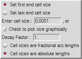
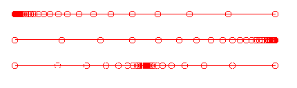
The user should set the desired location for specifying the cell size on the curve, either first end or last end. The user must then set the desired cell size at this location. This length may also be defined by picking a line segment graphically from the screen. If this mode of defining the cell length is chosen, the checkbutton should be set and the program will prompt for the input at the appropriate time. If a value is entered in the window, the user should use the final set of radiobuttons to indicate whether the number entered should be interpreted as an absolute distance value for the length of the cell or a fractional value defining the size of the cell relative to the total arc length of the curve or edge being regridded. The Decay Factor is also required, and determines how quickly the transition from a hyperbolic tangent to a hyperbolic sine function occurs. The three curves below show the results of regridding a line with 31 points, with a cell size of .001 of the total arc length, applied at the first end and last end, with a decay factor of 1. and again at the first end but with a decay factor of 2.
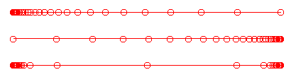
The geometric progression distribution function is used to set a fixed cell size at one or both ends of the curve or edge, and distribute the remaining points such that the cell lengths grow or shrink by a geometric progression. This function requires several additional inputs as shown in the window below. These buttons appear at the bottom of the list of distribution functions for any side whose option is set to "Geometric Progression".
Depending on which checkbuttons are set, the user should enter the desired cell size for each end of the curve. These lengths may also be entered by picking a line segment graphically from the screen. If this mode of defining the cell lengths is chosen, the checkbuttons should be set and the program will prompt for the inputs at the appropriate time. If values are entered in the window, the user should use the final set of radiobuttons to indicate whether the numbers entered should be interpreted as absolute distance values for the length of the first cell or fractional values defining the size of the first cell relative to the total arc length of the curve or edge being regridded. The three curves below show the results of regridding a line with 31 points, with a cell size of .001 of the total arc length, applied at the first end, last end, and at both ends.
The match existing distribution function is used to regrid a curve or surface edge to match a distribution function on an existing grid line. This is often used when a surface abuts a different surface which has already been regridded to achieve a certain grid distribution. This edge may even be the result of combining different distribution functions by joining curves or surfaces that have been distributed independently. If the matching distribution function is set, the program will prompt the user to graphically select a grid line on the screen to match the distribution on. The following set of radiobuttons is presented at the bottom of the list of distribution functions for any side whose option is set to "Match Existing Distribution".
If the grid line being matched has points running in the opposite direction from the curve being regridded, it may be necessary to specify with these radiobuttons that the distribution function should be reversed before being applied.
Note that for the Matching distribution function, the user may enter a 0 for the number of points to distribute. In this case, the program will automatically use the same number of points on the curve being regridded as exist on the gridline being matched to. If a non-zero value is entered, the program will compute the distribution function on the curve being matched to, and augment this function to the number of points specified.
The maintain existing distribution function is used to regrid a curve or surface edge using its own current distribution function, but with a new number of points. If the number of points requested is the same as already exist on the edge, an unchanged curve or edge will result. This is often desirable, when changing the distribution on side 1 of a surface but having side 3 remain unchanged. To maintain the current number of points, a 0 may be entered for the number of points when using the "Maintain Existing Distribution" option. If a non-zero value is entered, the program will augment the current function to the number of points specified.
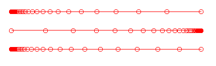
The four sine and cosine distribution functions are used to regrid a curve or surface edge using a pure sine or cosine function with the requested number of points. Depending on the option selected, points may be packed using this function at either the first end, last end, both ends, or in the middle of the curve. The four curves below show the results of distributing 31 points using the sine/cosine functions, at each of the four possible packing locations.
If the type of object being regridded is a surface, for Sides 3 and 4 the user has the option of simply selecting a "Same as Side 1" or "Same as Side 2" radio button, to apply the same distribution function as specified for the opposite side. This avoids the requirement for respecifying all the regridding inputs when the same function is to be applied all the way across a surface.
The image at the upper left below shows a simple square with 21 points in an equal arc distribution on each of the four sides. The additional images show the results of regridding this surface with 31 points, with varying distribution functions on the four sides. Examples include regridding only the grid lines in either of the directions, and regridding all four edges differently.

The text commands generated by the Regrid function are:
   om select {curve | surface} object_definition
   ggs set_dist {side1 | side2 | side3 | side4} diststring
where diststring is one of
   hyptan {[first s] [last s]} [method {absolute | relative}]
   geom {[first s] [last s]} [method {absolute | relative}]
   hypsin {[first s | last s | interior s loc s]} \
      [method {absolute | relative}]
   hybrid {[first s | last s]} [method {absolute | relative}] decay d
   sincos {first | last | both | interior}
   matching {forward | reverse}
   {equal | nochange | opposite}
and finally
   ggs redist dir {n | m | both} [interp {linear | nonlinear}] [n n] [m m]
   file save {default | name surfname}
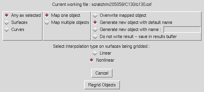
Selection of the "Map Surface or Curve onto Another ..." submenu causes the following window to be displayed.
Selection of the "Unstructured Mesh Quality ..." submenu causes the user to be prompted to select an unstructured object in the graphics window. After selecting the object, the following window is displayed.
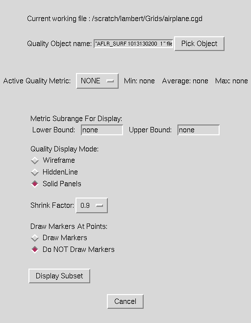
In this form, the user specifies the criteria for computing and displaying the quality of an unstructured mesh. Mesh quality on unstructured surface and volume meshes can be computed and displayed. The "Active Quality Metric:" drop down box is used to specify which quality metric should be computed. Depending on the type of object selected, surface and cell quality metrics may appear in this list. The only surface quality metric that is available is the "Minimum Edge Ratio". This metric is a measure of the ratio of the shortest edge over the longest edge in a face. Once a quality metric is selected, the minimum, maximum and average values for that metric will be listed beside the "Active Quality Metric" drop down box.
The user can now specify the options for display of the metric information. A subrange of the cells or faces to display is input in the "Metric Subrange For Display:" text entry boxes. Here the user can specify a lower and upper bound of the metric. Any faces/cells that fall within the specified range will be displayed when the "Display Subset" button is picked.
Example: For a case where the "Face Edge Ratio" quality metric provides a minimum value of 0.1, a maximum of 0.8 and an average of 0.7, specification of an "Upper Bound" of 0.2 will display all faces with a edge ratio between 0.1 and 0.2. Note that in this example, "none" is left in the "Lower Bound" text entry box to signify that no lower bound should be applied.
The "Quality Display Mode:" radio button boxes specify whether to draw the selected faces/cells in "Wireframe", "HiddenLine", or "Solid Panels" display mode.
The "Shrink Factor:" drop down box allows the user to specify a percentage to shrink the face/cell before displaying it. This option is useful for distinguishing individual cells for faces that touch each other.
The "Draw Markers At Points:" radio button specifies whether markers should be drawn at the nodes that make up each selected face or cell. This option is useful for highlighting the poor cells or faces in cases where they may otherwise not be visible. An example is the display of a triangular face that has collapsed to a degenerate edge. In this case, the face would appear as a single line and may be difficult to see or locate. By drawing the markers at the nodes, the face will be easier to see.
Once the metric has been selected and the display options specified, the "Display Subset" button will display the selected faces/cells. The options may be adjusted and the display updated by reselecting the "Display Subset" button at any time.
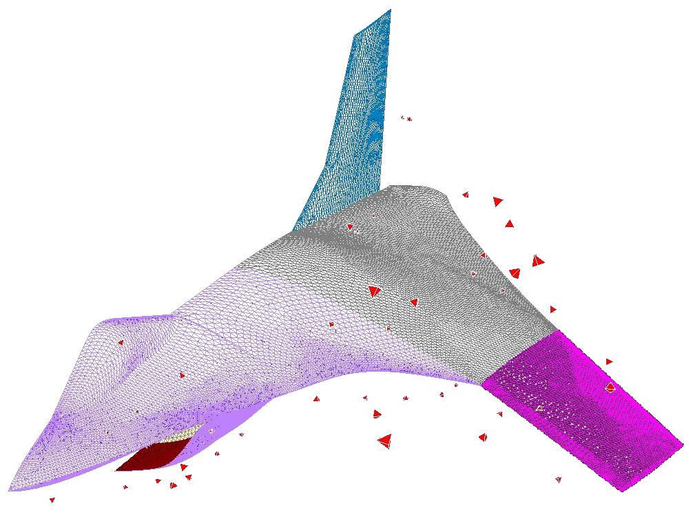
An example quality display for a cell quality metric is shown below.
Selection of the "2D Surface Elliptic ..." submenu causes the following window to be displayed.
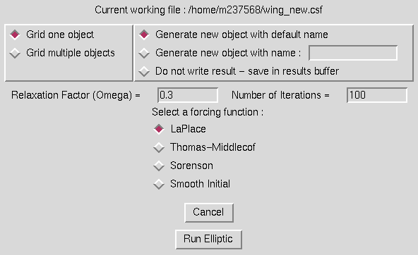
This operation is used to use elliptic smoothing to smooth the grid lines on a surface. Four methods are available for elliptic smoothing. LaPlace and Thomas-Middlecof smoothing require no further inputs beyong a relaxation factor (omega) and the number of iterations to run, both of which are entered in the entry boxes on the window. For the "Smooth Initial" function, additional inputs of an N- and M- subiteration count is also required (entry boxes will appear on the screen for these inputs). The most robust of the functions is the Sorenson. In this case, the window is modified as shown below.
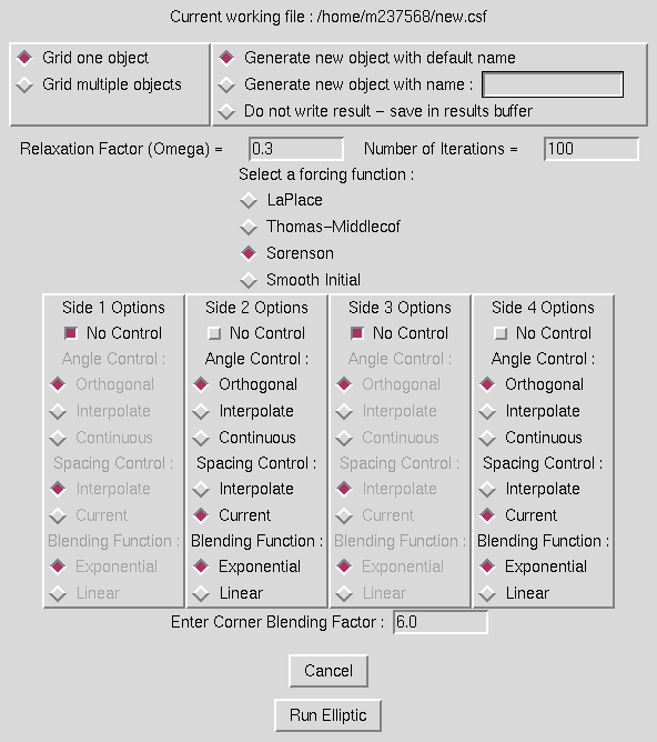
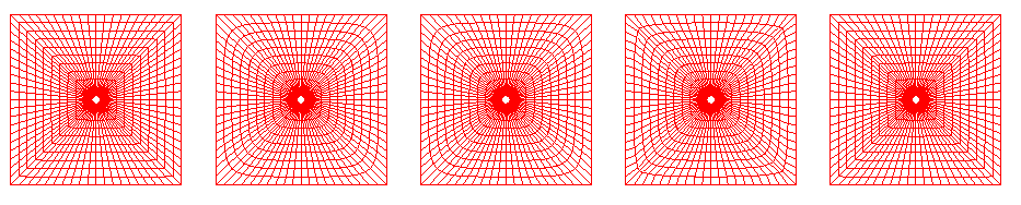
Under Sorenson elliptic smoothing, the user can control the angle grid lines approach edges, how the spacing off the wall is controlled from one end of an edge to the other, and how the options on different edges are blended near corners. These options can be independently specified on each of the four edges of a surface. A single corner blending factor is can also be set in the entry box at the bottom of the screen. The four images to the right below show the result of running elliptic smoothing on the typical polar grid inside a square region shown on the left. In order, the images are the results for LaPlace, Thomas Middlecof, Sorenson, and Smooth Initial elliptic options running 30 iterations with the default options.
When elliptic smoothing is run on a surface grid, the surface may be defined linearly or nonlinearly for interpolation purposes. After the "Run Elliptic" button is selected, the user will be prompted for the surface to smooth, and a new surface will be generated. This object should be specified as having a default name, a specified name, or to be saved in the results buffer. The text commands generated are:
om select surface surface_definitionfollowed by any of the following:
   elp set relaxation factor omega
   elp set forcing function 2d {laplace | middlecof | sorenson | smooth}
   elp set sorenson siden control {none | \
      angle {orthogonal | interpolate | continuous} \
      spacing {interpolate | current} blending_function {exponential | linear}}
   elp set sorenson blending_factor factor
   elp set smooth iterations {[mdir num] [ndir num]}
   elp elliptic [function {laplace | middlecof | sorenson | smooth}] \
      [interp {linear | nonlinear}] iterations iters
and finally
file save {default | name surfname}
Last updated 8 Dec 2008