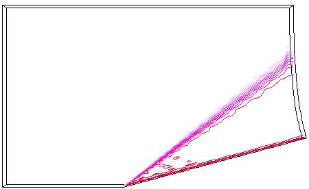
Figure 1. The shading of the Mach number for the Mach 2.5 flow
past a 15 degree wedge with the creation of an oblique shock.
Figure 1. The shading of the Mach number for the Mach 2.5 flow
past a 15 degree wedge with the creation of an oblique shock.
This study is an example study demonstrating the computational process for a supersonic flow past a wedge with a comparison of the results with analytical results. This study uses a three-dimensional flow domain and includes laminar and turbulent flow computations.
All of the archive files of this validation case are available in the Unix compressed tar file wedge03.tar.Z. The files can then be accessed by the commands
uncompress wedge03.tar.Z
tar -xvof wedge03.tar
A single-block, three-dimensional, structured grid was used for the flow domain. This grid is generated by extruding a planar grid into the z-direction. The planar grid is wedge2d.x.fmt. Fig. 2 shows this grid. The grid has 81 streamwise grid points with clustering near the leading edge of the wedge. The inviscid grid has 61 grid points in the transverse direction. The planar grid is extruded using the Fortran program x2d3d.f. The program is executed in the manner of
x2d3d < x2d3d.in
where x2d3d.in is a command file containing the name of the planar grid file. The program x2d3d extrudes the planar grid (planar in the x-y plane) in the z-direction from z = 0.0 to z = 12.0 inches using 5 evenly-spaced grid planes. The Fortran program gvisc (not provided here) is used to re-grid each j-grid line to apply a viscous spacing. The PLOT3D files resulting from this operation are listed in Table 1.
Table 1 presents information on the grids used in this study. The wall spacing is at the J1 boundary. The PLOT3D files are 3D, unformatted, multi-block, and in units of inches.
| Run | Grid Type | Grid Size | Wall Spacing (in) | Plot3d | FAST |
|---|---|---|---|---|---|
| A | - | - | - | - | - |
| B | Inviscid | 81 x 61 x 5 | 0.02 | wedge.B.x.dat | fast.B.x.com |
| C | Viscous | 81 x 71 x 5 | 1.0E-04 | wedge.C.x.dat | fast.C.x.com |
| D | Viscous | 81 x 71 x 5 | 1.0E-04 | wedge.D.x.dat | fast.D.x.com |
The Plot3d grid files are converted to the common grid (*.cgd) file format using the CFCNVT utility. This was done using the commands
cfcnvt < cfcnvt.B.com
cfcnvt < cfcnvt.C.com
cfcnvt < cfcnvt.D.com
where the files of the form cfcnvt.B.com are the command input files. Common grid files of the form cfcnvt.B.cgd are created.
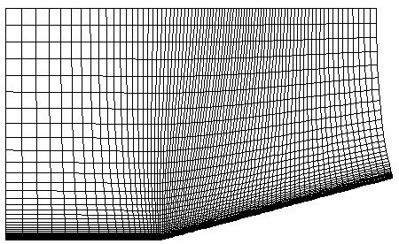
Figure 2. The grid for the 15 degree wedge.
An initial condition of freestream flow conditions is appropriate for this problem. Here, standard sea level conditions are used:
| Mach number | Static Pressure (psia) | Temperature(R) | Angle-of-Attack (deg) |
|---|---|---|---|
| 2.5 | 14.7 | 520.0 | 0.0 |
Since the inflow is supersonic, a FROZEN boundary condition can be applied at the I1 boundary. Since the outflow remains supersonic, except within the boundary layer, an extrapolation boundary condition is appropriate. This is imposed by specifying a CONFINED OUTFLOW boundary condition at the IMAX boundary. Within the input data file (i.e. wedge.B.dat) the downstream pressure will be specified to be extrapolated. Although this case is not an internal flow, the CONFINED OUTFLOW boundary condition can be used to impose the pressure boundary condition. The farfield boundary at JMAX is placed well above the oblique shock, and so, it can be specified with a FROZEN boundary condition. The K1 and KMAX boundaries are symmetry planes and so are specified with the INVISCID WALL boundary condition. The J1 boundary consists of a symmetry plane up to the leading edge of the wedge, which is at i = 21, and the wedge surface. The symmetry plane portion is specified as an INVISCID WALL boundary condition. The wedge surface is specified as a VISCOUS WALL boundary condition. This is done even if inviscid flow is to be computed. If inviscid flow is to be computed, then the inviscid keyword in the input data file (see wedge.B.dat) tells WIND that the viscous surface should be treated as a slip wall during the inviscid flow computation.
The boundary conditions can be interactively specified using GMAN. The procedure using the graphics interface is as follows:
1. Start GMAN.
gman
2. Read in the common grid file by typing at the GMAN prompt.
file wedge.B.cgd
3. Specify that units are inches.
units inches
4. Switch to graphics mode.
swi
5. Display the grid.
Pick SHOW (upper right panel)At this point the grid surface at k = 3 will be displayed. Moving the mouse so that the cross-cursor is near the upper-right most grid point and clicking the left mouse button will cause the coordinates of that point to be displayed in the middle right panel. It should indicate that the coordinates of point (81,61,1) are x = 67.0 in, y = 72.0 in, and z = 6.0 in. Note that the units are inches, which was desired from the units inches command.
GMAN defaults to zone 1 since it is the only zone. The sequence is to select the boundary and specify the boundary condition type on that boundary. The initial boundary condition type is UNDEFINED . GMAN is now waiting for the boundary to be specified.
Pick I1 (lower left panel)At this point, the I1 grid plane is displayed. Since the I1 grid plane is a constant-x grid plane, the view shows a line. Pressing on the left mouse button and moving the mouse to the right will turn the grid slightly to show the three-dimensional nature of the grid. To select the boundary condition type, execute the following menu choices
Pick MODIFY BNDYAt this point, the bottom panel should contain the text "305 points were changed". The boundary condition specification is now saved for this boundary by the following menu choices
Pick BOUNDARY COND. (top left panel)The common grid file wedge.cgd is modified to include this boundary condition specification.
The boundary condition specification can be checked by selecting
Pick IDENTIFY PNTS. (left panel)The individual grid points will show up in color to indicate that those points are specified as FROZEN .
The boundary conditions for the other boundaries are set in a similar manner. For the IMAX boundary,
Pick BOUNDARY COND. (top left panel)For the JMAX boundary,
Pick BOUNDARY COND. (top left panel)
Pick PICK ZONE/BNDY
Pick JMAX
Pick MODIFY BNDY
Pick CHANGE ALL
Pick FROZEN
Pick BOUNDARY COND.
Pick YES-UPDATE FILE
For the K1 boundary,
Pick BOUNDARY COND. (top left panel)
Pick PICK ZONE/BNDY
Pick K1
Pick MODIFY BNDY
Pick CHANGE ALL
Pick INVISCID WALL
Pick BOUNDARY COND.
Pick YES-UPDATE FILE
For the KMAX boundary,
Pick BOUNDARY COND. (top left panel)
Pick PICK ZONE/BNDY
Pick KMAX
Pick MODIFY BNDY
Pick CHANGE ALL
Pick INVISCID WALL
Pick BOUNDARY COND.
Pick YES-UPDATE FILE
As mentioned above, the J1 boundary contains two different boundary condition specifications. The symmetry plane extends from I1 to I21 and is specified as an INVISCID WALL boundary condition. The wedge surface extends from I21 to IMAX and is specified as a VISCOUS WALL boundary condition. The specification of the boundary conditions are done in GMAN in the following manner:
Pick BOUNDARY COND. (top left panel)
Pick PICK ZONE/BNDY
Pick J1
Now the sub-area representing the symmetry plane on the J1 boundary is identified and the boundary conditions are set just on that sub-area. The sub-area is set by using the menu items in the lower-right panel of the GMAN screen.
Pick Work Subarea (lower right panel)
GMAN will print a prompt in the bottom panel for inputs on the start and end of the K-I range for the sub-area. These can be typed in or picked from the grid display with the mouse.
Enter 1 1
Enter 5 20
The display in the lower right-hand panel will indicate that indices for the working sub-area just defined. The boundary conditions are specified as previously:
Pick MODIFY BNDY
Pick CHANGE ALL
Pick INVISCID WALL
Pick BOUNDARY COND.
Pick YES-UPDATE FILE
If one picks the IDENTIFY PNTS. item, one can see that only the grid points on the symmetry plane were changed to INVISCID WALL . Now the wedge surface is identified as a sub-area and the boundary conditions are specified as VISCOUS WALL .
Pick Work Subarea (lower right panel)
Enter 1 21
Enter 5 81
Pick MODIFY BNDY
Pick CHANGE ALL
Pick VISCOUS WALL
Pick BOUNDARY COND.
Pick YES-UPDATE FILE
Pick TOP (top left panel)
Pick END
Pick YES-TERMINATE
The common grid file wedge.B.cgd is now ready.
As GMAN operates, a journal file gman.jou is created which can later be used as a command file to re-run GMAN. Here this file has been renamed gman.B.com and GMAN can be re-run as
gman < gman.B.com
Creating a command file from scratch represents an alternative to the graphical approach within GMAN.
| Run | GMAN Command File | Common Grid File |
|---|---|---|
| A | - | - |
| B | gman.B.com | wedge.B.cgd |
| C | gman.C.com | wedge.C.cgd |
| D | gman.D.com | wedge.D.cgd |
The computation strategy involves starting from the freestream solution and marches in time using local time-stepping until the L2 residual has leveled off. A constant CFL number of 5.0 is used.
The first three lines of the input data file are comment lines describing the case and file. (i.e. see wedge.B.dat).
The freestream keyword lists the static freestream conditions for the Mach number, pressure in psia, temperature in degrees Rankine, angle-of-attack in degrees, and angle-of-sideslip in degrees.
The inviscid keyword in the input data file wedge.B.dat indicates that viscosity is not to be computed. The laminar keyword in the input data file wedge.C.dat indicates that laminar flow is to be computed. The turbulence keyword in input data file wedge.D.dat indicates that turbulent flow is to be computed using the Baldwin-Lomax turbulence model.
The downstream pressure keyword indicates that the confined outflow boundary in zone 1 is to always be extrapolated.
The cycles keyword indicates the number of cycles that are to be run. The iterations per cycle keyword indicates the number of iterations to be be run for each cycle.
The cfl keyword indicates that the CFL number is constant at 5.0.
| Run | Input Data File | Viscosity | Cycles | Iterations / Cycle |
|---|---|---|---|---|
| A | - | - | - | - |
| B | wedge.B.dat | Inviscid | 1 | 300 |
| C | wedge.C.dat | Laminar | 3 | 500 |
| D | wedge.D.dat | Baldwin-Lomax | 3 | 500 |
The WIND solver is run by entering
wind
WIND displays interactive prompts for appropriate information for the input data file and output file names. Table 5 presents the CPU times and output files for each run.
| Run | CPU (sec) | List File | Solution File |
|---|---|---|---|
| A | - | - | - |
| B | 176.19 | wedge.B.lis | wedge.B.cfl |
| C | 3673.99 | wedge.C.lis | wedge.C.cfl |
| D | 3789.14 | wedge.D.lis | wedge.D.cfl |
In runs C and D, it was noticed that some messages were printed in the list files of the form.
ltdsolv: singular matrix at n=2. tdbtri: singular matrix: l= 22
The exact cause of these messages is not clear; however, a reduction of the CFL number may eliminate the messages. Regardless, the solution seems to be computed fine.
Information on the convergence history of the L2 residual can be obtained from the list files (i.e. wedge.B.lis) using the utility RESPLT,
resplt < resplt.B.com
resplt < resplt.C.com
resplt < resplt.D.com
The file resplt.B.com is a command file containing the inputs for resplt to output the GENPLOT file nsl2.B.gen containing the residual history data. The program CFPOST can now be used to read in nsl2.B.gen and plot the convergence history.
cfpost < cfpost.B.nsl2.com
cfpost < cfpost.C.nsl2.com
cfpost < cfpost.D.nsl2.com
| Run | RESPLT File | GENPLOT File | CFPOST File |
|---|---|---|---|
| A | - | - | - |
| B | resplt.B.com | nsl2.B.gen | cfpost.B.nsl2.com |
| C | resplt.C.com | nsl2.C.gen | cfpost.C.nsl2.com |
| D | resplt.D.com | nsl2.D.gen | cfpost.D.nsl2.com |
Fig. 3 shows a plot of the residual data.
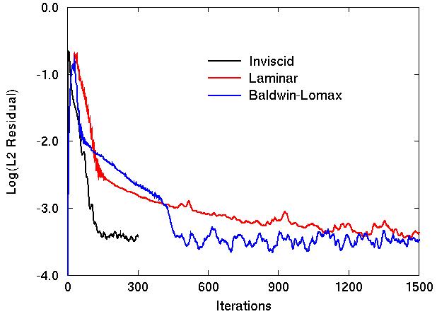
Figure 3. Plot of the L2 residual history.
The PLOT3D solution files can generated from CFPOST by the following commands:
cfpost < cfpost.B.plot3d.com
cfpost < cfpost.C.plot3d.com
cfpost < cfpost.D.plot3d.com
where cfpost.B.plot3d.com is the command input file. The PLOT3D solution file is wedge.B.q.dat. This is written using the standard PLOT3D non-dimensionalization. Fig. 1 shows the Mach number contours for the solution. The files are unformatted, single-block, and three-dimensional.
| Run | CFPOST Command File | PLOT3D Solution File | FAST Script File |
|---|---|---|---|
| A | - | - | - |
| B | cfpost.B.plot3d.com | wedge.B.q.dat | fast.B.q.com |
| C | cfpost.C.plot3d.com | wedge.C.q.dat | fast.C.q.com |
| D | cfpost.D.plot3d.com | wedge.D.q.dat | fast.D.q.com |
The pressure distribution along the symmetry and wedge surfaces (J1 boundary) can be output by CFPOST using the commands:
cfpost < cfpost.B.pres.com
cfpost < cfpost.C.pres.com
cfpost < cfpost.D.pres.com
where cfpost.B.pres.com is the command input file. The distribution is written to the GENPLOT data file presx.B.gen. Fig. 4 compares this distribution to the theoretical solution, which is listed in the data file presx.theory.
| Run | CFPOST Command File | GENPLOT File |
|---|---|---|
| A | - | - |
| B | cfpost.B.pres.com | presx.B.gen |
| C | cfpost.C.pres.com | presx.C.gen |
| D | cfpost.D.pres.com | presx.D.gen |
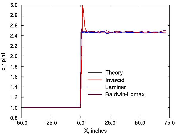
Figure 4. Comparison of the pressure distribution along
the J1 boundary.
The distribution compares well; however, for the inviscid run, there is a significant overshoot at the leading edge of the wedge.
These computations were performed on an Silicon Graphics Power Challenger using one single R10000 194 MHZ IP25 Processor. The CPU times are presented in Table 5.
Information on this case can be obtained from:
John W. Slater
NASA Glenn Research Center, MS 86-7
21000 Brookpark Road
Cleveland, Ohio 44111
Phone: (216) 433-8513
e-mail: John.W.Slater@grc.nasa.gov