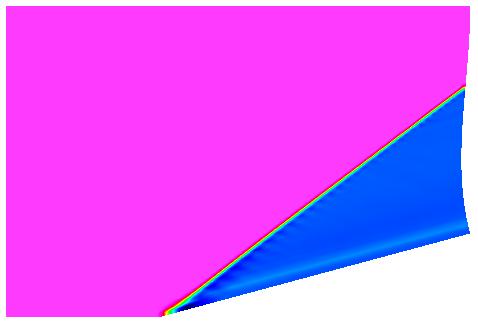
Figure 1. The shading of the Mach number for the Mach 2.5 flow
past a 15 degree wedge with the creation of an oblique shock.
Figure 1. The shading of the Mach number for the Mach 2.5 flow
past a 15 degree wedge with the creation of an oblique shock.
This study performs a grid convergence study of the WIND code for solving a simple supersonic flow past a wedge. Comparisons are made between the computed results and analytic results from theory.
All of the archive files of this validation case are available in the Unix compressed tar file wedge02.tar.Z. The files can then be accessed by the commands:
uncompress wedge02.tar.Z
tar -xvof wedge02.tar
Single-block, two-dimensional, structured grids were generated for the flow domain. The computational grids were approximately a uniformly spaced for most of the flowfield. An example image of the grid is shown in Fig. 2 below.
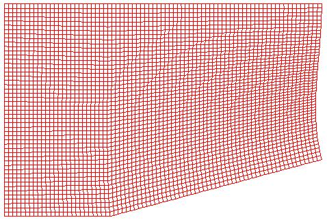
Figure 2. A plot of a representative grid for the wedge.
The table below lists the names of the common grid files (*.cgd) and the Plot3D files (*.x.bin) for the grids. The Plot3d files are three-dimensional, whole, single-block and binary.
| Grid | Spacing | Density | CGD File | Plot3d Grid File |
|---|---|---|---|---|
| A | 0.02 | 78 x 51 | wedge.A.cgd | wedge.A.x.bin |
| B | 0.01 | 155 x 101 | wedge.B.cgd | wedge.B.x.bin |
| C | 0.005 | 308 x 201 | wedge.C.cgd | wedge.C.x.bin |
| D | 0.0031 | 496 x 324 | wedge.D.cgd | wedge.D.x.bin |
An initial condition of freestream flow conditions is appropriate for this problem. Here, standard sea level conditions are used:
| Mach number | Static Pressure (psia) | Temperature(R) | Angle-of-Attack (deg) |
|---|---|---|---|
| 2.5 | 14.7 | 520.0 | 0.0 |
An INVISCID WALL boundary condition is applied at the J1 boundary to apply appropriate inviscid flow conditions at both the symmetry plane and the surface of the wedge. Since the inflow is supersonic, a FROZEN boundary condition can be applied at the I1 boundary. Since the outflow remains supersonic an extrapolation boundary condition is appropriate. This is imposed by specifying a INFLOW OUTFLOW boundary condition at the IMAX boundary. Within the input data file the downstream pressure at the outflow boundary will be specified to be extrapolated. The farfield boundary at JMAX is placed well above the oblique shock, and so, it can be specified with a FROZEN boundary condition.
The boundary conditions are specified using an input command file with GMAN run in batch mode,
gman < gman.wedge.A.com
gman < gman.wedge.B.com
gman < gman.wedge.C.com
gman < gman.wedge.D.com
The computation strategy is starts from the freestream solution and marches in time using local time-stepping until the L2 residual has leveled off. A constant CFL number of 5.0 is used.
Table 2 below lists the input data files that were used for each run.
The steady-state flow was computed for each grid. Table 2 lists the names of the input data files for each run (picking the file name will cause the ASCII file to be displayed). The runs mostly used the default input values for WIND. A CFL number of 5.0 was used for all runs. The computations were performed for a set number of iterations until that the convergence histories leveled out.
| Grid | Input Data File | CFL Number | Iterations | CPU Time (sec) |
|---|---|---|---|---|
| A | wedge.A.dat | 5.0 | 500 | 204.10 |
| B | wedge.B.dat | 5.0 | 300 | 846.43 |
| C | wedge.C.dat | 5.0 | 500 | 5948.52 |
| D | wedge.D.dat | 5.0 | 1500 | 48866.00 |
| Grid | List File | CFL File | Plot3d Solution | L2 Residual | Mach -vs- x |
|---|---|---|---|---|---|
| A | wedge.A.lis | wedge.A.cfl | wedge.A.q.bin | wl2a.do | wmxa.do |
| B | wedge.B.lis | wedge.B.cfl | wedge.B.q.bin | wl2b.do | wmxb.do |
| C | wedge.C.lis | wedge.C.cfl | wedge.C.q.bin | wl2c.do | wmxc.do |
| D | wedge.D.lis | wedge.D.cfl | wedge.D.q.bin | wl2d.do | wmxd.do |
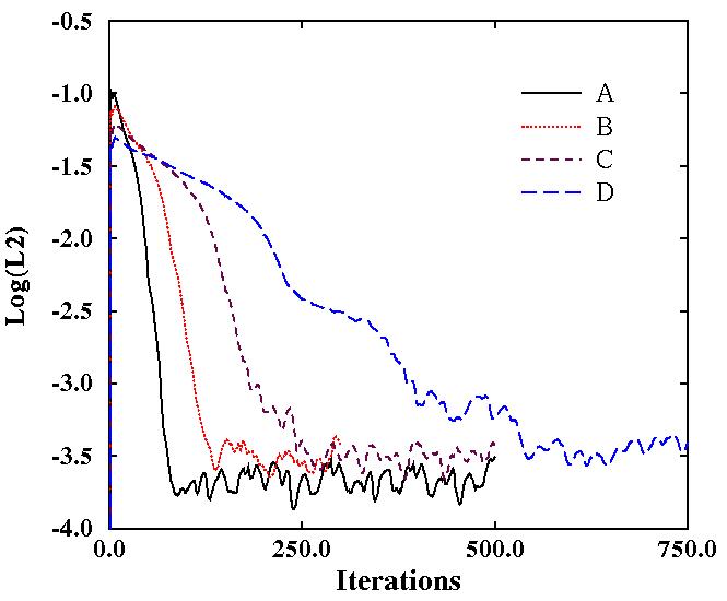
Figure 3. The plots of the convergence histories for the
WIND computations of the Mach 2.5 flow past a 15 degree wedge.
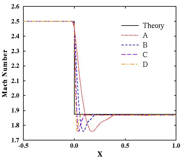
Figure 4. The plots of the Mach number distributions
along the wedge surface as compared to theory.
Since the exact solution is known for the entire flowfield, the errors in the computed solution can be evaluated. Table 4 presents those errors for each grid. The Total Error is the area-weighted average of the sum of the absolute differences between the computed conservation variables and the exact conservation variables at each solution point. The Total Mach Error is the area-weighted average of the difference between the computed Mach number and the exact Mach number at each solution point. The Average Mach Number is the area-weighted average of the Mach number behind the shock. The Mach Error is the error in percent of the average Mach number behind the shock to the exact Mach number.
| Grid | Total Error | Total Mach Error | Average Mach | Mach Error (%) |
|---|---|---|---|---|
| A | 2.8394E-02 | 1.7019E-05 | 1.8809 | 0.3911 |
| B | 7.2166E-03 | 3.0962E-06 | 1.8765 | 0.1590 |
| C | 1.8251E-03 | 5.6126E-07 | 1.8748 | 0.0655 |
| D | 7.0310E-04 | 1.7111E-07 | 1.8742 | 0.0371 |
Since the exact solution for the flowfield is known and the errors are computed above with respect to several grid sizes, it is possible to determine the order of accuracy of WIND for this application. The order of accuracy is determined as the slope of the data plotted as Log( Total Error ) versus Log( ds ) where ds is the grid spacing. For the four grids, a linear regression was performed to determine the slope of the data which was 1.98344. Thus it can be said that this computation was calculated with second-order spatial accuracy.
The grid convergence study examines the convergence of the solution as the grid is refined. The approach of Roach is followed in conducting the study. The observed quantity used for the study was the average Mach number behind the shock as presented as Average Mach in Table 4 above. Table 5 presents the results of the grid convergence study and reports on the values of the grid convergence index (GCI). The GCI values are quite low, which suggests that all the grids are within the asymptotic range of grid spacings. This is evident when one sees that the errors in the average Mach numbers as presented in Table 4 are quite low.
| Grid | Spacing | r | Average Mach | epsilon | GCI(%) |
|---|---|---|---|---|---|
| A | 0.02 | 2 | 1.8809 | 2.3181E-03 | 0.9272 |
| B | 0.01 | 2 | 1.8765 | 9.3345E-04 | 0.3734 |
| C | 0.005 | 1.6129 | 1.8748 | 2.8438E-04 | 0.1386 |
| D | 0.0035 | - | 1.8742 | - | - |
The amount of CPU time required for each computation is shown in Table 2.
Roache, P.J., "Perspective: A Method for Uniform Reporting of Grid Refinement Studies", Journal of Fluids Engineering , Vol. 116, September 1994.
Information on this case can be obtained from:
John W. Slater
NASA Glenn Research Center, MS 86-7
21000 Brookpark Road
Cleveland, Ohio 44111
Phone: (216) 433-8513
e-mail: John.W.Slater@grc.nasa.gov