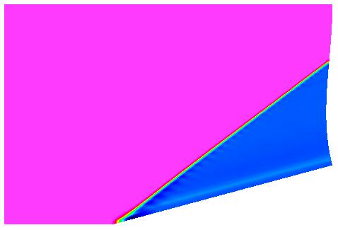
Figure 1. The shading of the Mach number for the Mach 2.5 flow
past a 15 degree wedge with the creation of an oblique shock.
Figure 1. The shading of the Mach number for the Mach 2.5 flow
past a 15 degree wedge with the creation of an oblique shock.
This study is an example stud demonstrating the computational process using a simple supersonic flow past a wedge with a comparison of the results with analytical results.
All of the archive files of this validation case are available in the Unix compressed tar file wedge01.tar.Z. The files can then be accessed by the commands
uncompress wedge01.tar.Z
tar -xvof wedge01.tar
A single-block, two-dimensional, structured grid was generated for the flow domain. The grid points are uniformly spaced with a grid spacing of 0.01 ft. This results in a grid density of 155 streamwise and 101 transverse grid points. The Plot3d grid file (formatted, single-block, two-dimensional, double-precision) is wedge.x.fmt. Fig. 2 shows the grid.
The Plot3d grid file was converted to the common grid file (*.cgd) format using the CFCNVT utility. This was done using the command:
cfcnvt < cfcnvt.wedge.com
where the file cfcnvt.wedge.com is a command input file (standard Fortran input unit). A common grid file named wedge.cgd is created.
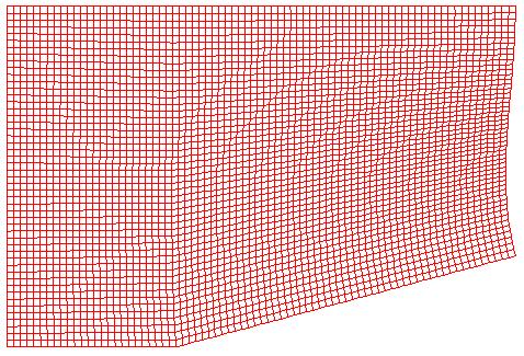
Figure 2. The grid for the 15 degree wedge (grid has been
coarsened for viewing.
An initial condition of freestream flow conditions is appropriate for this problem. Here, standard sea level conditions are used:
| Mach number | Static Pressure (psia) | Temperature(R) | Angle-of-Attack (deg) |
|---|---|---|---|
| 2.5 | 14.7 | 520.0 | 0.0 |
An INVISCID WALL boundary condition is applied at the J1 boundary to apply appropriate inviscid flow conditions at both the symmetry plane and the surface of the wedge. Since the inflow is supersonic, a FROZEN boundary condition can be applied at the I1 boundary. Since the outflow remains supersonic an extrapolation boundary condition is appropriate. This is imposed by specifying a CONFINED OUTFLOW boundary condition at the IMAX boundary. Within the input data file, wedge.dat, the downstream pressure will be specified to be extrapolated. Although this case is not an internal flow, the CONFINED OUTFLOW boundary condition can be used to impose the pressure boundary condition. The farfield boundary at JMAX is placed well above the oblique shock, and so, it can be specified with a FROZEN boundary condition.
The boundary conditions are specified using GMAN. The procedure using the graphics interface is as follows:
gman
file wedge.cgd
units fss
swi
Pick SHOW (upper right panel)
Pick SHOW SURFACES
Pick PICK K-PLANE
At this point the grid will be displayed since there is only one grid plane, k=1. Moving the mouse so that the cross-cursor is near the upper-right most grid point and clicking the left mouse button will cause the coordinates of that point to be displayed in the middle right panel. It should indicate that the coordinates of point (155,101,1) are x = 1.0 ft, y = 1.0 ft, and z = 1.0 ft. Note that the units are feet, which was desired from the units fss command. Also note that CFCNVT had converted the initial two-dimensional grid to a three-dimensional grid with z = 1.0 ft, which is required by WIND.
Pick BOUNDARY COND. (left panel)
GMAN defaults to zone 1 since it is the only zone. The sequence is to select the boundary and specify the boundary condition type on that boundary. The initial boundary condition type is UNDEFINED . GMAN also defaults to picking a zone and picking zone 1. It is now waiting for the boundary to be specified.
Pick I1 (lower left panel)
At this point, the I1 grid plane is displayed. Since this case is planar, a line is displayed. To select the boundary condition type, execute the following menu choices
Pick MODIFY BNDY
Pick CHANGE ALL
Pick FROZEN
At this point, the bottom panel should contain the text "101 points were changed". The boundary condition specification is now saved for this boundary by the following menu choices:
Pick BOUNDARY COND. (top left panel)
Pick YES-UPDATE FILE
The common grid file wedge.cgd is modified to include this boundary condition specification.
The boundary condition specification can be checked by selecting:
Pick IDENTIFY PNTS. (left panel)
Pick FROZEN
The individual grid points will show up in color to indicate that those points are specified as FROZEN .
The boundary conditions for the remaining three boundaries are set in a similar manner. For the IMAX boundary,
Pick BOUNDARY COND. (top left panel)
Pick PICK ZONE/BNDY
Pick IMAX
Pick MODIFY BNDY
Pick CHANGE ALL
Pick CONFINED OUTFLOW Pick BOUNDARY COND.
Pick YES-UPDATE FILE
For the J1 boundary,
Pick BOUNDARY COND. (top left panel)
Pick PICK ZONE/BNDY
Pick J1
Pick MODIFY BNDY
Pick CHANGE ALL
Pick INVISCID WALL Pick BOUNDARY COND.
Pick YES-UPDATE FILE
For the JMAX boundary,
Pick BOUNDARY COND. (top left panel)
Pick PICK ZONE/BNDY
Pick JMAX
Pick MODIFY BNDY
Pick CHANGE ALL
Pick FROZEN
Pick BOUNDARY COND.
Pick YES-UPDATE FILE
Pick TOP (top left panel)
Pick END
Pick YES-TERMINATE
The common grid file wedge.cgd is now ready.
As GMAN operates, a journal file gman.jou is created which can later be used as a command file to re-run GMAN. Here this file has been renamed gman.wedge.com and GMAN can be re-run as:
gman < gman.wedge.com
Creating a command file from scratch represents an alternative to the graphical approach within GMAN.
The computation strategy is starts from the freestream solution and marches in time using local time-stepping until the L2 residual has leveled off. A constant CFL number of 5.0 is used.
The input data file is wedge.dat. The first three lines are comment lines describing the case and file.
The freestream keyword lists the static freestream conditions for the Mach number, pressure in psia, temperature in degrees Rankine, angle-of-attack in degrees, and angle-of-sideslip in degrees.
The inviscid keyword indicates that viscosity is not to be computed.
The downstream pressure keyword indicates that the confined outflow boundary in zone 1 is to always be extrapolated.
The cycles keyword indicates that only 1 cycle will be run. The iterations per cycle keyword indicates that 500 iterations will be run for that 1 cycle.
The cfl keyword indicates that the CFL number is constant at 5.0.
The WIND solver is run by entering:
wind
Some initial interactive prompts ask for information to set up the computation. First, select 1 to run the Production version .
Running command line version of WIND.


                   ***** WIND Run Script *****


Current wind settings are:

--Wind test mode set to NODEBUG
--Wind debugger set to DEFAULT
--Wind run que set to PROMPT
--Wind run in place mode is set to NO
--Wind multi-processor mode set to NO
--Wind run directory set to PROMPT
--Wind bin directory set to /net/zargon/usr2/wind-1.0/wind

                 Select the desired version

  0: Exit wind
  1: Production version

Enter number or name of executable.......[1]: 1
The next question will ask for the name of the input data file. Enter the name without the "dat" file extension. So, for this case, enter:
wedge
Enter number or name of executable.......[1]: 1
Basic input data................(*.dat): wedge
The next few questions ask about "Output data", "Mesh file", and "Flow data file" file names. Entering a carriage return will select the default names. A common flow data file wedge.cfl does not currently exists, so WIND initialize the flow from the freestream conditions and creates a the new flow data file.
Output data.............(*.lis,=wedge): Mesh file...............(*.cgd, =wedge): Flow data file..........(*.cfl, =wedge): *********************************************************** wedge.cfl does not exist, a fresh start will be performed. ***********************************************************
The next question allows a choice between running the solution in real-time (interactive) or submitting it to a queue. First, try running it interactively by selecting 1 .
Enter a queue number from the following list orfor default: 1: REAL (interactive) 2: AT_QUE Queue name.......................( for 1):
The next question asks about the remote directory. Enter a return.
# Note the remote directory is assumed to exist on remote host # Enter the remote run root directory...(for /tmp):
The next questions asks whether the output should be written to the screen or to a list file wedge.lis . Enter n to create a list file.
Print output at screen?....................(y/n,=y): n
Some file information will be printed.
Version...............: /net/zargon/usr2/wind-1.0/wind/SGI5/R4400/windprod.exe
Input file name.......: wedge.dat
Wind output to........: wedge.lis
Grid file name........: wedge.cgd
Flow file name........: wedge.cfl
Job run que type is...: REAL
A final carriage return will cause the job to be submitted.
Pressto submit job, another key (except space) and to abort:
This computation was performed on an Silicon Graphics Iris Indigo workstation with a single R4000 100 MHZ IP20 Processor and 80 MB of main memory.
The list file is wedge.lis and contains the output from the computation and lists the residual information for all of the iterations. The flow data file is wedge.cfl and contains the final solution.
Information on the convergence history of the L2 residual can be obtained from the list file wedge.lis using the utility RESPLT,
resplt < resplt.wedge.com
The file resplt.wedge.com is a command file containing the inputs for resplt to output the file wedge.resl2.gen containing the residual history data.
The program CFPOST can now be used to read in wedge.resl2.gen and plot the convergence history.
cfpost < cfpost.wedge.resl2.com
Fig. 3 shows a plot of the residual data. As can be seen, the residual drops less than three orders of magnitude and levels off in about 200 iterations.
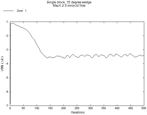
Figure 3. Plot of the L2 residual history.
The PLOT3D grid and solution files can generated from CFPOST by the following command:
cfpost < cfpost.wedge.plot3d.com
where cfpost.wedge.plot3d.com is the command input file. The PLOT3D grid file is wedge.x.dat and the solution file is wedge.q.dat. These are written using the standard PLOT3D non-dimensionalization. Fig. 1 shows the Mach number contours for the solution. The files are unformatted, single-block, and three-dimensional.
The Mach number distribution along the symmetry and wedge surfaces (J1 boundary) can be output by CFPOST using the command:
cfpost < cfpost.wedge.mach.com
where cfpost.wedge.mach.com is the command input file. The distribution is written to the GENPLOT data file wedge.mach.gen. Fig. 4 compares this distribution to the exact solution, which is listed in the data file wedge.mach.exact.
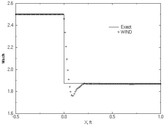
Figure 4. Comparison of the Mach number distribution along
the J1 boundary.
The distribution compares well; however, there is a significant overshoot at the leading edge (corner for this case).
The static pressure, density, and temperature distributions along the J1 boundary can be output from the data file using CFPOST using the command:
cfpost < cfpost.wedge.prhoT.com
where cfpost.wedge.prhoT.com is the command input file. The distributions are written to the GENPLOT data file wedge.prhoT.gen. Table 2 compares the WIND results at the last grid point on the wedge surface (i=155, j=1) with the analytic results. As can be seen, the comparisons are very good.
| Property | Theory | WIND | Error(%) |
|---|---|---|---|
| Mach number behind the oblique shock | 1.873526 | 1.868440 | -0.271 |
| Pressure ratio (p2/p1) | 2.467500 | 2.469570 | 0.084 |
| Density ratio (rho2/rho1) | 1.866549 | 1.856064 | -0.562 |
| Temperature ratio (T2/T1) | 1.321958 | 1.330541 | 0.649 |
The computation of this case required 1453 CPU seconds to run 500 iterations with one cycle. Fig. 3 indicates that perhaps only 200 iterations are needed for convergence. A second computation was performed for 200 iterations and required 580 CPU seconds. A check on the Mach number distribution showed no change from the 500 iteration computation, thus 200 iterations are adequate for convergence.
Information on this case can be obtained from:
John W. Slater
NASA Glenn Research Center, MS 86-7
21000 Brookpark Road
Cleveland, Ohio 44111
Phone: (216) 433-8513
e-mail: John.W.Slater@grc.nasa.gov