

| a. |
b. |
|---|
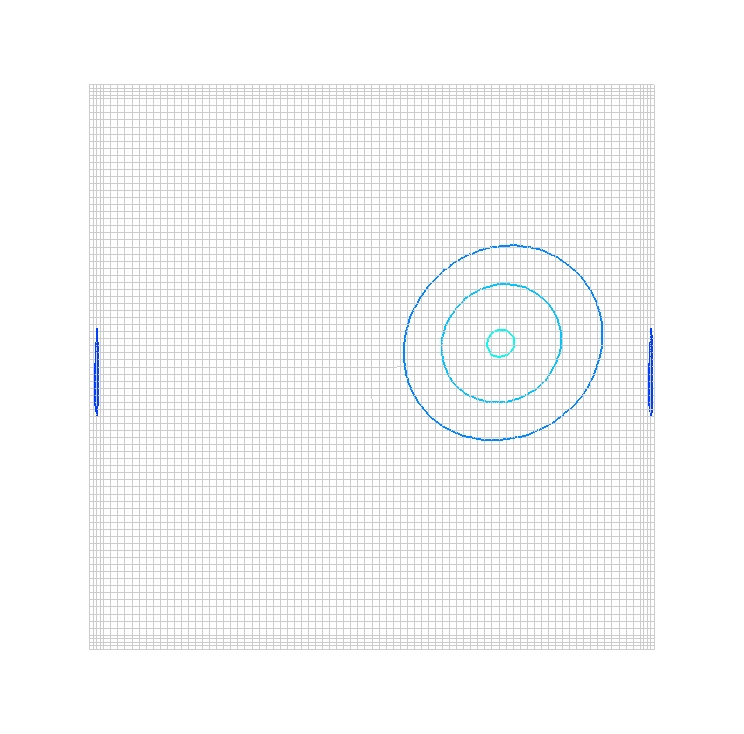
Figure 1. Vorticity profiles for an inviscid convected vortex.
| a. |
b. |
|---|
Figure 1. Vorticity profiles for an inviscid convected vortex.
In this test case, an inviscid vortex is convected through a square domain with periodic boundary conditions. The initial position of the vortex is in the center of the grid, as shown in Figure 1a. The vortex has strength &Gamma = 5 and is allowed to convect downstream in Mach 0.5 flow with a nondimensinal time step of 0.1. The vorticity of the vortex is described by &omega = [&Gamma(2-R)/2&pi]{exp[0.5(1-R)]}, where R = (x-x0)2 + (y-y0)2, and x0 and y0 describe the vortex center. The grid is given periodic boundary conditions in the flow direction, which is from left to right. The vortex should complete one flow cycle on the grid every 200 time steps.
All of the archive files of this validation case are available in the Unix compressed tar file vortex01.tar.Z. The files can then be accessed by the commands
uncompress vortex01.tar.Z
tar -xvof vortex01.tar
The grid is generated by the program mkgrid.f, which generates an 85x85x1 grid with uniform spacing with the exception of the outer boundaries, where the spacing is halved to allow for use of the double fringe boundary condition. The resulting grid is a Plot3d file (formatted, single-zone, whole, three-dimensional) named mkgrid.fmt.x.
The Plot3d grid file is converted to the common grid file (*.cgd) format using the CFCNVT utility. This is done using the command
cfcnvt < cfcnvt.x.com
where the file cfcnvt.x.com is a command input file (standard Fortran input unit). A common grid file named vortex.cgd is created.
The initial flow conditions are generated by the program makeq.f, which generates the initial vortex on the above grid, mkgrid.fmt.x and writes a Plot3d solution file (formatted, single-zone,whole, three-dimensional) named vortexic.fmt.q for the initial solution. This Plot3d solution file is converted to the common solution file (*.cfl) format using the CFCNVT utility. This is done using the command
cfcnvt < cfcnvt.q.com
where the file cfcnvt.q.com is a command input file (standard Fortran input unit). A common flow file named vortexic.cfl is created.
The boundary conditions are set within the common grid file vortex.cgd. The boundary conditions on the upper and lower boundaries are set to INVISCID; on the left and right boundaries, they are set to DOUBLE FRINGE. The GMAN utility is used with the following command
gman < gman.com
where the file gman.com is a command input file (standard Fortran input unit). This process updates common grid file vortex.cgd to include the boundary conditions.
The computation is performed using the time-marching capabilities of Wind-US to march in a time-accurate manner to simulate the unsteady flow. For each time step, a constant global physical time step is used throughout the entire flowfield. Five individual runs are computed. The default full block implicit (left-hand-side) operator is used for all runs, with either first order (default) or second order time marching specified. The Global Newton iteration technique, aimed at stabilizing the solution and improving time accuracy, is also used for some of the runs; for each Global Newton iteration, the convergence order is 5 with either 3 or 5 subiterations specified. Table 2, below, summarizes these five runs.
| Run | Implicit Order | Global Newton Iterations |
|---|---|---|
| A | 2 | 5 |
| B | 1 | 5 |
| C | 1 | 0 |
| D | 2 | 0 |
| E | 2 | 3 |
The input data files for the five Wind-US runs described above are named vortex.A.dat, vortex.B.dat, vortex.C.dat, vortex.D.dat and vortex.E.dat. All input parameters are identical for each run, except where noted below. The freestream keyword indicates that the static freestream flow conditions are specified as Mach number, pressure (psia), temperature (R), angle-of-attack (degrees), and angle-of-sideslip (degrees). The turbulence keyword indicates that flow is inviscid. The converge keyword indicates that the solution will automatically stop if the maximum residual is less than 1.0e-09. The implicit keyword specifies the full block implicit time integration scheme to be used in all directions. The implicit order keyword sets the order of the implicit time marching scheme to either one or two as indicated in Table 2, above. The implicit boundary keyword specifies that implicit boundary conditions within the implicit solver are to be used on the inviscid wall boundaries. The rhs keyword specifies that the second-order upwind-biased Roe scheme modified for stretched grids is to be used. The cfl# keyword specifies that the time step calculation procedure originally used in the OVERFLOW code is used; the run is specified to be time accurate and the time step in seconds nondimensionalized by Lr / ar is 0.1.
For runs C and D, the cycles keyword specifies that 1000 cycles are to be computed and the iterations keyword specifies that there is to be 1 iteration per cycle.
For runs A, B and D, the newton keyword indicates that the Global Newton time stepping algorithm is to be used to advance 1000 Global Newton time levels with the convergence order set to 5. Within a Newton time level, the iterations keyword specifies 1 iteration per cycle. The cycles keyword specifies 3 cycles for run E which effectively results in three subiterations per Global Newton iteration. For runs A and B, the five subiterations are specified.
The input data files also specify that 2 processes are spawned (or begun) at the specified time level intervals for each case. The first process spawned is a shell script named save_cfl.sh which writes out the cfl files at the specified time intervals. The second process spawned is a shell script named min_rho_p_loc.sh which tells CFPOST to write out the grid and solutions files as temporary files in plot3d format, and then use them as input into the Fortran77 program min_rho_p_loc.f which computes the minimum density, pressure and the x,y,z location of the minimum pressure for the current time level. This information is then written to an output file.
The directories named runA, runB, runC, runD and runE were created for each case. Within each directory, the Wind-US solver is run by entering
wind -runinplace -dat vortex.N -list vortex.N -flow vortex.N -grid ../vortex
where N is the run identifier ( A, B, C, D or E). Further details and options for the wind script can be found in the WIND-US documentation (wind script).
As Wind-US is computing each run, several output files are generated, and these files are tabulated in Table 3, below. An output list file (.lis) is created which contains the output from the computation including the residual information. The flow field solution files (.cfl) after each 200 time levels. To save disk space, only the flow files from the final solution at the last time step are included. A file which contains the minimum density, pressure and location of the minimum pressure, resulting from the spawned process min_rho_p_loc.sh, is also included for each run.
| Run | List | Flow | Min rho & p data |
|---|---|---|---|
| A | vortex.A.lis | vortex.A.cfl | min_rho_p_loc.A.trace |
| B | vortex.B.lis | vortex.B.cfl | min_rho_p_loc.B.trace |
| C | vortex.C.lis | vortex.C.cfl | min_rho_p_loc.C.trace |
| D | vortex.D.lis | vortex.D.cfl | min_rho_p_loc.D.trace |
| E | vortex.E.lis | vortex.E.cfl | min_rho_p_loc.E.trace |
The utility CFPOST was used to write out the grid and solution results in Plot3d format. The cfpost command files for accomplishing this are cfpost.p3d.A.com, cfpost.p3d.B.com, cfpost.p3d.C.com, cfpost.p3d.D.com and cfpost.p3d.E.com. To run cfpost for runA, for example, the following command was used:
cfpost < cfpost.p3d.A.com
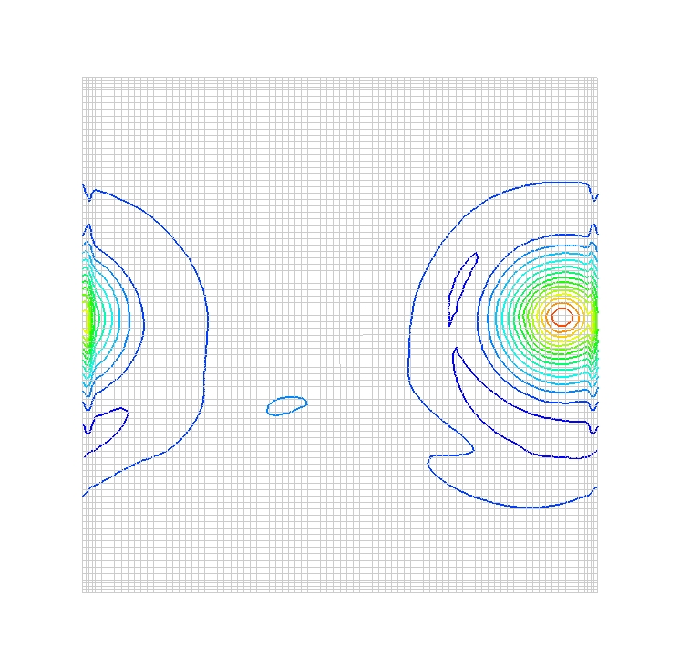
The resulting Plot3d grid file is named vortex.x, and the Plot3d solution files for each case are named vortex.A.5000.q, vortex.B.5000.q, vortex.C.1000.q, vortex.D.1000.q and vortex.E.3000.q. These files were read by the post processing program Fieldview, to obtain the vorticity contour plots shown below in Figure 2. (Note: The full grid was used for all calculations, although several lines appear missing in Figure 2 as a result of importing the graphics.)


| a. |
b. |
|---|
| c. |
d. |
|---|

e. Figure 2. Vorticity profiles at the final time step.
The post processing for the quantities of interest for this problem was accomplished through the spawned process min_rho_p_loc.sh, which is spawned at the specified time intervals during the Wind-US runs, as described above. The process runs the program min_rho_p_loc.f, minimum density and pressure, and the location of the minimum pressure. As mentioned above, this data is then written to the respective min_rho_p_loc.N.trace file. The results were also written in Tecplot ASCII "point" format, with corresponding files named min_rho_p_loc.N.dat, then Tecplot was used to create the plots below.
This first set of comparisons looks at first and second order time marching, with and without the Global Newton iteration technique used. For the vertical vortex location, the vortex should move horizontally across the grid, with no change in vertical position. As shown in Figure 3, runs A and B which used Global Newton iteration, best accomplished this.
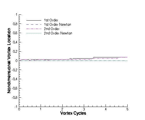
Figure 3. Vertical location of the vortex minimum pressure. Global Newton cases used 5 subiterations.
The minimum pressure in the vortex should essentially stay constant in time. The vortex should remain the same shape and size, but simply move across the domain. As Figure 4 indicates, the 2nd-order methods maintain the smallest overall change in pressure. The change is less when the Global Newton iteration scheme is omitted, however, the pressure values are slightly oscillatory.
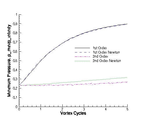
Figure 4. Vortex minimum pressure. Global Newton cases used 5 subiterations.
For the density, both 2nd-order methods give similarly good values, both again, the case which used the Global Newton scheme was smoother.
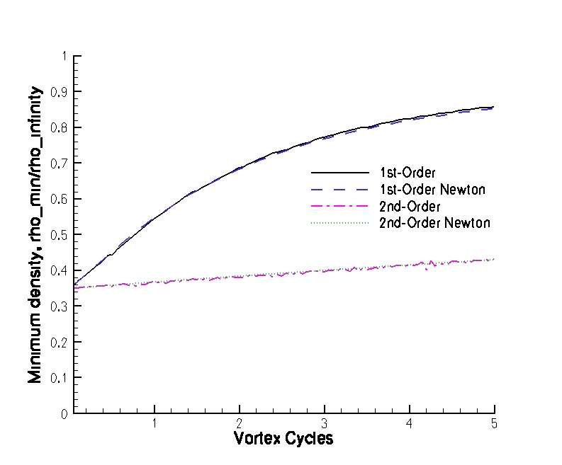
Figure 5. Vortex minimum density. Global Newton cases used 5 subiterations.
As Figures 6 through 8 below indicate, using Global Newton Iteration gives slight improvement in the vertical location of the minimum pressure and smooths out the minimum pressure and density values. There is not much to be gained by using 5 subiterations rather than 3 subiterations.

Figure 6. Vertical location of the vortex minimum pressure. 2nd order time marching is used and the number of Global Newton subiterations is varied.

Figure 7. Vortex minimum pressure. 2nd order time marching is used and the number of Global Newton subiterations is varied.
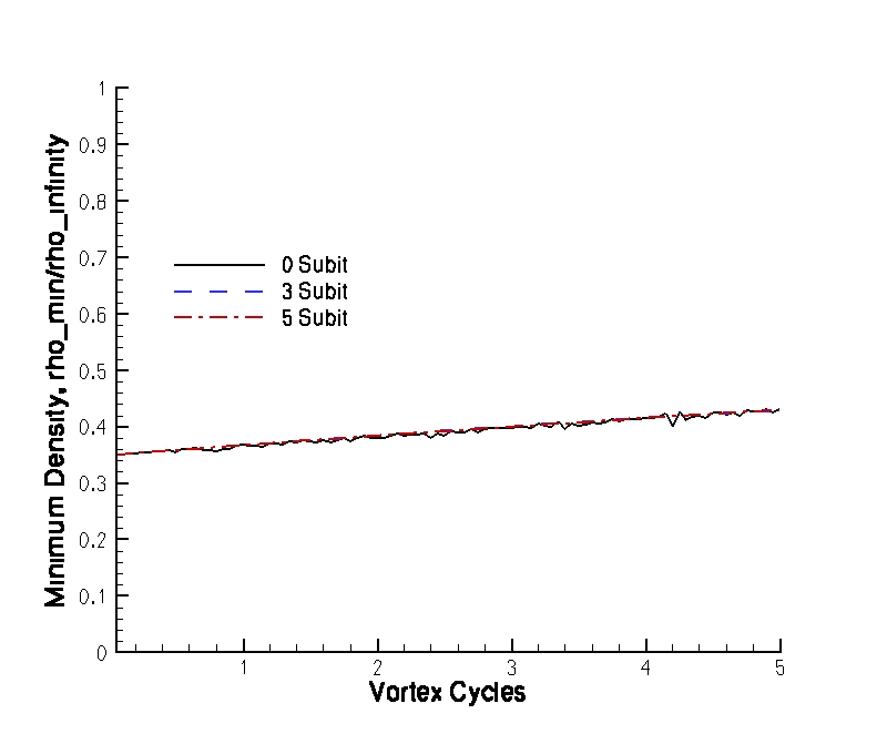
Figure 8. Vortex minimum density. 2nd order time marching is used and the number of Global Newton subiterations is varied.
This case was run using Wind-US alpha version 2.94 on an HP xw6200 workstation running the LINUX operating system. The computational times for each case are given in Table 4.
| Run | Implicit Order | Global Newton Iterations | Total No. of Iter (Incl. Newton Subiters.) | Total CPU Time (sec) |
|---|---|---|---|---|
| A | 2 | 5 | 5000 | 401 |
| B | 1 | 5 | 5000 | 386 |
| C | 1 | 0 | 1000 | 85.17 |
| D | 2 | 0 | 1000 | 86.01 |
| E | 2 | 3 | 3000 | 247 |
This case was created on March 13, 2006 by Chris Nelson, who may be contacted at
Innovative Technology Applications Company, LLC
Phone: (425) 778-7853
e-mail: Chris Nelson
and Julianne C. Dudek, who may be contacted at
NASA John H. Glenn Research Center, MS 86-7
21000 Brookpark Road
Brook Park, Ohio 44135
Phone: (216) 433-8513
e-mail: Julianne.C.Dudek@nasa.gov