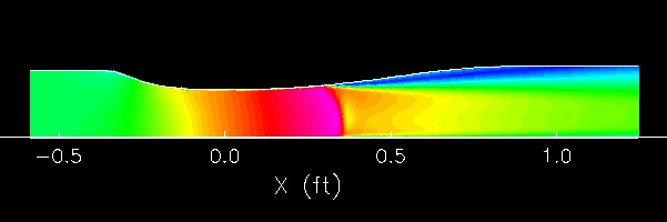
Figure 1. Mach number contours for the Strong Shock
case of the Sajben transonic diffuser.
Figure 1. Mach number contours for the Strong Shock
case of the Sajben transonic diffuser.
This validation study examines the use of the unstructured flow solver in Wind-US for simulating transonic flow through a diffuser with adverse pressure gradients and shock-induced separation. The "Strong Shock" flow condition is used.
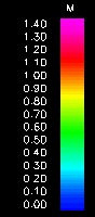
The grid is an unstructured hexahedral version of the 2-D structured grid used in Study #1, Study #2, and Study #3 and is shown in Figure 2. Since the unstructured solver requires volume cells, the 2-D grid was extruded two inches into the third dimension, spanned by one grid cell. Expressed as a structured grid, the dimensions became 81 x 51 x 2. To create the unstructured representation, the I/J/K indices were replaced by a single index.
The grid spacing at the wall is approximately 2.0E-04 inches. This wall spacing results in turbulent boundary layers being resolved to a y+ of approximately 2.
The grid is contained in the the common grid file sajben_s2u.cgd .
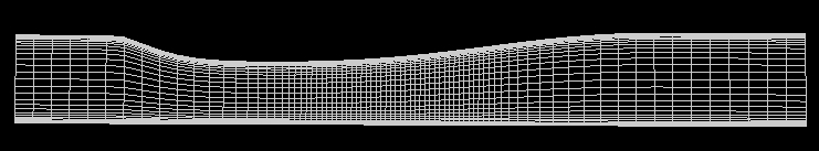
Figure 2. Side view of the unstructured hexahedral grid
for the Sajben transonic diffuser.
Boundary conditions were selected to generate the Strong Shock case described in Study #2 . On the inflow boundary (on the left in the images), an ARBITRARY INFLOW boundary condition was imposed using a total pressure of 19.5 psi and total temperature of 500 R. The outflow boundary had an OUTFLOW BC with 14.1 psi static pressure imposed. The upper and lower boundaries were viscous walls. The Singular Axis BC was imposed on the two sidewalls (parallel to the page) in order to avoid the needless computation of pressure fluxes normal to the boundary that would be computed by an inviscid wall BC but which are unecessary since the side walls are flat and parallel to the flow.
Wind-US 1.115 was used to compute the flow solution. The modified Rusanov upwind scheme was selected because it is the preferred unstructured solver in Wind-US for most problems. Local time stepping with a CFL number of 10 was used to converge on a steady-state solution. The Spalart-Allmaras turbulence model was used.
Two runs were made, each using a different combination of smoothing inputs and convergence criterion. For the first run, the two smoothing input parameters were set to minimal reasonable strengths in order to provide the greatest solution accuracy. SECOND, which is the upwind flux dissipation, was set to 0.1. SMLIMT, which is the TVD slope limiter, was set to 4.0. (Note that FOURTH is the the Jacobian dissipation and should always remain set to 1.5.) The run was stopped when the L2 residuals of both the Navier-Stokes solver and the turbulence model were seen to have visibly flattened.
The second run made use of the Wind-US unstructured solver's automatic convergence capability, referred to as the "CONVERGE LOADS" strategy because it is activated using the CONVERGE LOADS keywords in the DAT input file. Wind-US automatically sets and adjusts the smoothing input parameters (SECOND and SMLIMT), reducing their strengths as the loads converge. The run is stopped automatically when Wind-US detects that the pressure loads and viscous loads have converged. In this study, the loads were integrated over the upper and lower viscous walls.
The initial flow conditions were identical to the inflow condition: uniform Mach 0.9 flow in the x-direction at a total pressure of 19.5 psi and total temperature of 500 R.
The following two input files were used in this study. Each file is thoroughly commented.
| Run | Smoothing Control | Convergence Criterion | Input Data File |
|---|---|---|---|
| 1 | manual | enough iterations for L2 to converge | sajben_s2u.dat.run1 |
| 2 | automatic | auto detection of loads convergence | sajben_s2u.dat.run2 |
Wind-US is run on a single processor on a UNIX computer by entering a command like so:
wind -runinplace sajben_s2u.cgd
The names of the output list file and the solution file for each run are listed in Table 2.
| Run | Output List File | Solution File |
|---|---|---|
| 1 | sajben_s2u.lis.run1 | sajben_s2u.cfl.run1 |
| 2 | sajben_s2u.lis.run2 | sajben_s2u.cfl.run2 |
Runs 1 and 2 each examine iterative convergence their own way as described in the Computational Strategy section above.
Run 1 - Residual of the Navier-Stokes solver and turbulence model
The L2 norm of the residual of the Navier-Stokes equations can be read from the output list file. The residuals are read and plotted in the following procedures:
resplt < resplt.L2.com
cfpost < cfpost.L2.com
Figure 3 shows the solution residual of Run 1 that is displayed by CFPOST.
Figure 3. Plot of the L2 norm of Navier-Stokes residuals for
Run 1.
Figure 4 shows the residual of the S-A model of Run 1 that is displayed by CFPOST.
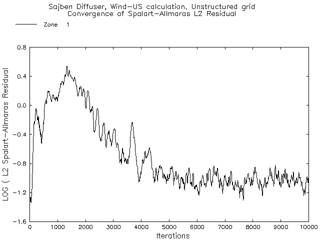
Figure 4. Plot of the L2 norm of Spalart-Allmaras residuals for
Run 1.
Run 2 - Automatic "CONVERGE LOADS" strategy
The CONVERGE LOADS keywords make Wind-US automatically set and adjust the smoothing parameters, monitor the pressure and viscous loads, and automatically halt the calculation when the loads converge. A plot of these loads can be produced using the following procedure:
resplt < resplt.cvglds.com
cfpost < cfpost.cvglds.com
Figure 5 shows the convergence of the viscous loads of Run 2 that is displayed by CFPOST.
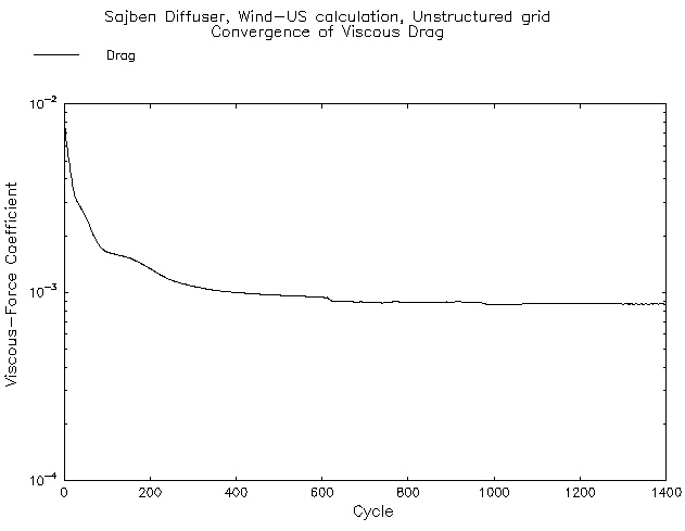
Figure 5. Plot of the viscous loads for Run 2.
The CFPOST utility can be used to generate information from the the data files. The scripts and images below are for Run 1, but look identical to those for Run 2.
Mach Number Contour Plots. The CFPOST utility can be used to generate and plot Mach number contours of the planar flow,
cfpost < cfpost.mach.com
Figure 1 at the top of this page shows the contour plot for Run 1.
Table 3 provides GENPLOT files containing experimental data. These files must be present for the CFPOST scripts below to include experimental data in the plots.
| Description | File |
|---|---|
| top wall static presssures | p.top.gen.exp |
| bottom wall static presssures | p.bot.gen.exp |
| velocity profile at x = 5" | u.x0.gen.exp |
| velocity profile at x = 8" | u.x1.gen.exp |
| velocity profile at x = 11" | u.x2.gen.exp |
| velocity profile at x = 13" | u.x3.gen.exp |
Static Pressure Distributions. The distribution of the static pressures on the top and bottom of the diffusers can be obtained using CFPOST like so:
cfpost < cfpost.ptop.com
cfpost < cfpost.pbot.com
These operations create the GENPLOT files of the static pressure distributions.
Figures 6-7 show the resulting plots.
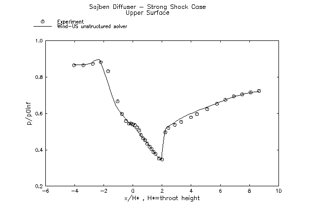
Figure 6. Static pressure distribution along the top wall
of the diffuser.
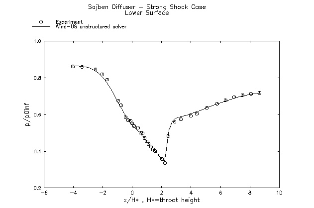
Figure 7. Static pressure distribution along the bottom wall
of the diffuser.
Velocity Profiles. The velocity profiles at axial stations along the diffuser can be compared to experimental data using CFPOST like so:
cfpost < cfpost.u.com
These operations create the GENPLOT files of the velocity distributions in the vertical direction at axial stations at x-coordinates of 5.0 inches, 8.0 inches, 11.0 inches, and 13.0 inches. (the throat is at 0 inches).
Figures 8-11 show the resulting plots.
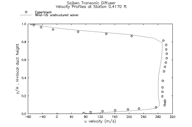
Figure 8. Plot of the u-velocity profile at
x = 5.0 inches (Run 1).
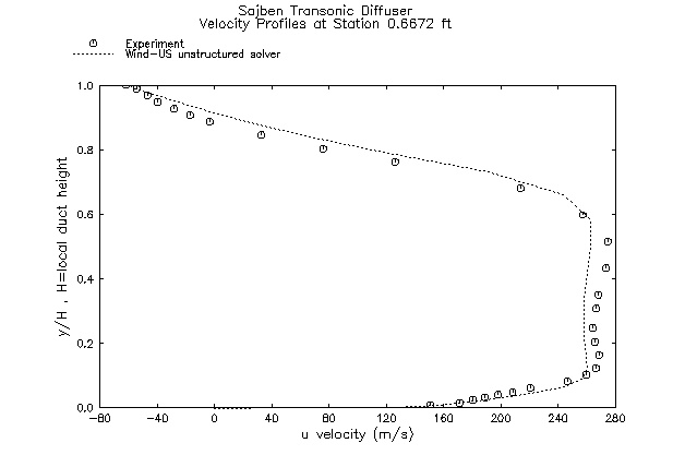
Figure 9. Plot of the u-velocity profile at
x = 8.0 inches (Run 1).
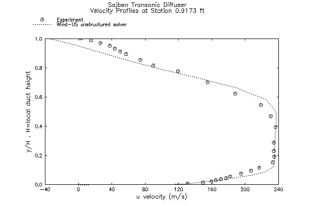
Figure 10. Plot of the u-velocity profile at
x = 11.0 inches (Run 1).
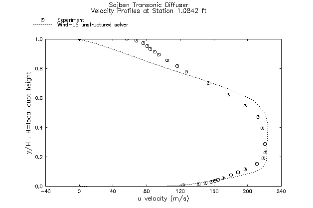
Figure 11. Plot of the u-velocity profile at
x = 13.0 inches (Run 1).
Static Pressure Distributions. Figures 6 and 7 show the static pressure distributions along the top and bottom of the diffuser and they indicate generally good agreement with the experimental data. Run 2, not pictured, looked identical to Run 1.
Velocity Profiles. Figures 8 through 11 show the comparison of the u-velocity profiles at the axial stations for Run 1. The agreement between Wind-US and experiment is generally good, but diminishes toward the downstream stations. This disagreement may be due to 3-D effects seen in the experiment. The calculation could not reproduce 3-D effects because the grid did not model or resolve any spanwise characteristics of the duct. Also, a more advanced turbulence model might produce better agreement.
Run 2, not pictured, looked identical to Run 1.
Further details of this study are described in the following paper, available online:
Mohler, S.R., "Wind-US Unstructured Flow Solutions for a Transonic Diffuser," NASA CR-2005-213417, January 2005
This study was last updated on April 14, 2005 by Stan Mohler Jr., who may be contacted at:
Stan.Mohler@grc.nasa.gov