This study is an model study comparing the accuracy and performance of the shock tube computations from WIND with those of NPARC.
All of the archive files of this validation case are available in the Unix compressed tar file stube02.tar.gz. The files can then be accessed by the commands
gunzip stube02.tar.gz
tar -xvof stube02.tar
The grid for the WIND and NPARC computations is planar and evenly-spaced with 100 axial grid points and 21 radial grid points.
For WIND, the Fortran program stubegr.f generates the grid and outputs the Plot3d file (formatted, single-block, whole, two-dimensional) named stube.x.fmt. This file is converted to the common grid file (*.cgd) format using the CFCNVT utility,
cfcnvt < cfcnvt.x.com
where the file cfcnvt.x.com is a command input file (standard Fortran input unit). A common grid file named stube.cgd is created.
For NPARC, the Fortran program sodic.f generates the grid and outputs it to the restart file fort.2.
The initial flow conditions are stationary flow with different pressure and density values on each side of the diaphragm. The diaphragm is located at x = 0.5 ft (grid index I = 50). A 10/1 pressure is specified with the static pressure and temperature values given in Table 1, below.
| Region | Pressure (psia) | Temperature (R) |
|---|---|---|
| 1 | 1.0 | 416.0 |
| 4 | 10.0 | 520.0 |
In Wind-US, the initial flow conditions are specified in the input data file, stube02.dat, as described later.
For NPARC, the Fortran program sodic.f also generates the initial solution outputs it to the restart file fort.2.
For both WIND and NPARC, the INVISCID WALL boundary condition is applied at the J1 and JMAX boundaries of the grid. The FROZEN boundary condition is applied at the I1 and IMAX boundaries of the grid.
For WIND, the boundary conditions are specified using GMAN,
gman < gman.com
where gman.com is the command file.
For NPARC, the boundary conditions are specified within the input data file sodst3.in. The FROZEN boundary conditions are Type -10 and the INVISCID WALL boundary conditions are Type 50.
Both computations are performed using the time-marching capabilities to march in a time-accurate manner to simulate the unsteady flow. A constant time step is specified to be used for each time step. The number of time steps is specified such that the desired time interval is spanned.
The input data file for WIND is stube02.dat. The keyword inviscid indicates that the inviscid flow is assumed. The axisymmetric keyword indicates that the flow domain is assumed to be axisymmetric with a waterline of 0.0 feet and a degree of rotation of 5 degrees. The arbitrary inflow keyword block indicates that the static conditions described in Table 1, above, are to be used, with the higher pressure in the upstream half of the shock tube. The stages keyword indicates that the four-stage Jameson-type of Runge-Kutta time integration algorithm is to be used. The implicit none keyword indicates that the time integration is to be explicit. The cycles and iterations keywords indicate that one cycle with 500 time steps is to be run. The timesteps keyword indicates that the actual time step in seconds is specified.
The input data file for NPARC is sodst3.in. The IVARDT keyword indicates that a constant, uniform time step with the non-dimensional value of DTCAP was used. The NMAX keyword indicates that 500 time steps were used. The DIS2 keyword indicates the level of second-order smoothing. The ISOLVE keyword indicates that the four-stage Runge-Kutta solver was used. The IAXISY keyword indicates that axisymmetric flow is assumed.
The Wind-US computation was performed on an HP xw9400 workstation with dual-core 2599 MHZ AMD Opteron Processor and 896 MB of main memory. Only one processor was used. The list file is stube02.lis and contains the output from the computation and lists the residual information for all of the iterations. The flow data file is stube02.cfl and contains the final solution.
The NPARC computation was performed on a Silicon Graphics Octane workstation with two R10000 195 MHZ IP30 Processors and 896 MB of main memory. Only one processor was used. The output was directed to the file sodst3.out. The file fort.4 contains the final solution; however, for this problem, the needed output is already in the file sodst3.out.
Since the WindUS and NPARC cases were run on different computers, a comparison of their computational time is not given.
For the WINDUS solution, the CFPOST utility was used to generate the data files for the distributions of the pressure, density, velocity, and Mach number along the shock tube.
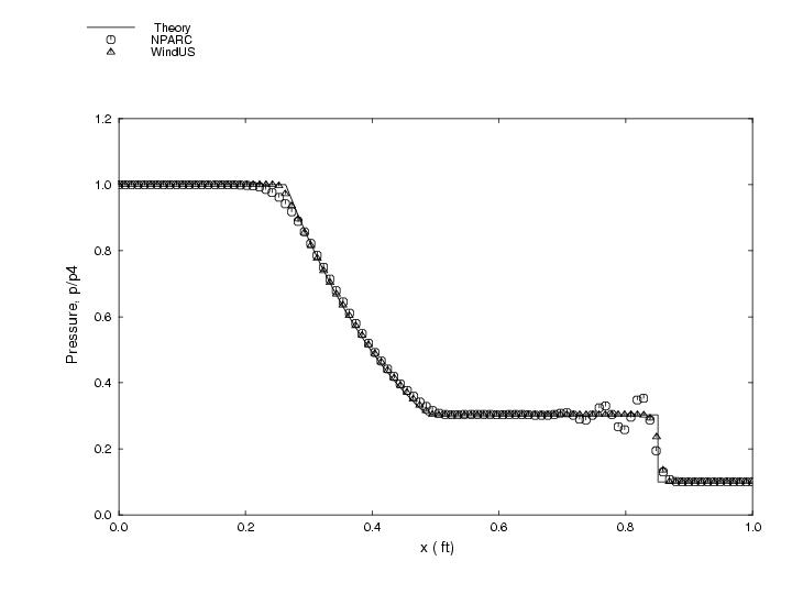
The following CFPOST files compute the pressure, density and Mach number, respectively, from the WindUS solution: cfpost.p.com, cfpost.rho.com, and cfpost.mach.com. They also generate corresponding GENPLOT files of the results named p.gen, rho.gen, and mach.gen. So, for example, to create the pressure plot in Figure 1, the following procedure is used.First the pressure is calculated and the p.gen GENPLOT file is written by executing CFPOST:
cfpost < cfpost.p.com
Then another CFPOST command file, cfpost.p_comp.com, is used to plot these Wind-US results with the NPARC result (p.nparc.gen) and the theoretical result (p.theory.gen).
cfpost < cfpost.p_comp.com
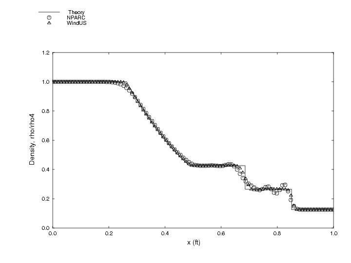
The results are shown in Figure 1, below. Similarly, the density along the shock tube is calculated as follows.
cfpost < cfpost.rho.com
Then the CFPOST command file, cfpost.rho_comp.com is used to plot these Wind-US results for density with the NPARC result (rho.nparc.gen) and the theoretical results contained in the GENPLOT file rho.theory.gen.
cfpost < cfpost.rho_comp.com
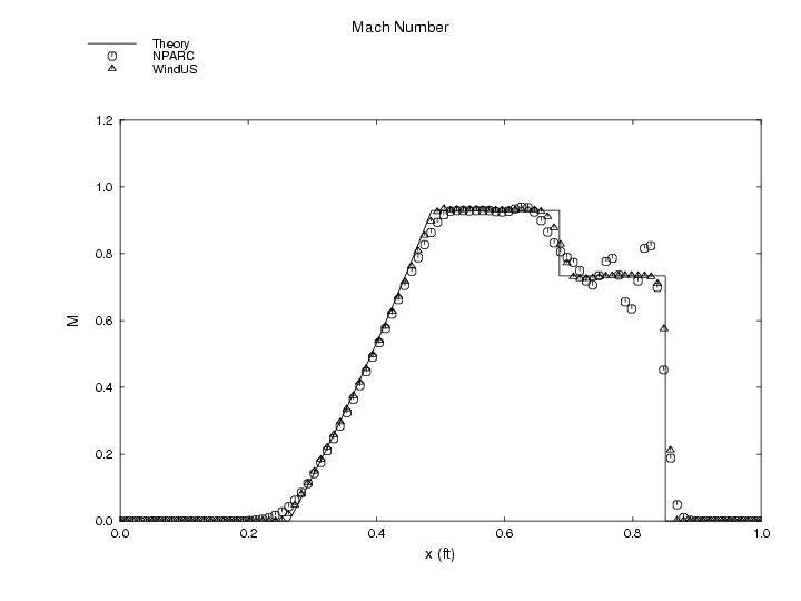
These results are shown in Figure 2, below. Similarly, the Mach number along the shock tube is calculated as follows.
cfpost < cfpost.mach.com
Then the CFPOST command file, cfpost.mach_comp.com is used to plot these Wind-US results for density with the NPARC result (mach.nparc.gen) and the theoretical results contained in the GENPLOT file mach.theory.gen.
cfpost < cfpost.mach_comp.com
Thses results are shown in Figure 3, below.