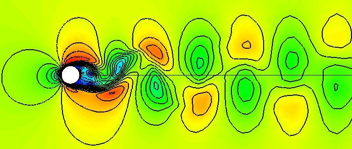
Figure 1. Mach number contours.
Figure 1. Mach number contours.
This study examines laminar flow over a circular cylinder. The incoming freestream flow is uniform with a Mach number of 0.2 and a Reynolds number based on diameter of 150. At this Reynolds number, the flow is essentially two dimensional with periodic vortex pairs shed from the downstream side of the cylinder. 1, 2 Solutions computed using the full block implicit scheme with the first and second order operators specified are compared with solutions in which the Global Newton time stepping has also been specified. The drag coefficient and Strouhal number are compared with the experimental data of Roshko.2
All of the archive files of this validation case are available in the Unix tar file cyl_lam_s.tar. The files can then be accessed by the commands:
tar -xvof cyl_lam_s.tar
A structured C-grid was used with 401 points in the circumferential direction and 201 points in the radial direction. The grid is contained in the Wind grid file cyl_lam_s.cgd. The cylinder diameter is 1.0 meter, with the J1 boundary at the cylinder wall, where the wall spacing is 1.044E-03 meters; this corresponds to a maximum y+ of approximately 0.06. The JMAX boundary is the far-field boundary and is located 200 diameters from the center of the cylinder. The I1 and IMAX boundaries are coincient at the downstream side of the cylinder and are aligned with the freestream flow; the progression from I1 to IMAX is in the clockwise direction.
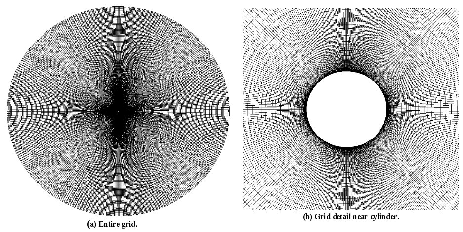
Figure 2. Computational Grids
The initial conditions are uniform flow at the freestream conditions which are given in Table 1 below. These conditions correspond to a Reynolds number of 150 based on the cylinder diameter of 1.0 meter.
| Mach number | Static Pressure (psia) | Temperature(R) | Angle-of-Attack (deg) |
|---|---|---|---|
| 0.2 | 0.00045146 | 500.0 | 0.0 |
The boundary conditions must now be specified for the grid, and this may be done using the GMAN utility. The boundary conditions are specified as follows: a VISCOUS WALL boundary is specified on the J1 boundary, a FREESTREAM condition is specified on the JMAX boundary, and boundaries I1 and IMAX are COUPLED to each other.
The boundary conditions can be set either by running GMAN in an interactive mode or by creating an input data file and running GMAN in batch mode. The input file gman.com was created and gman was executed in batch mode as shown.
gman < gman.com
The computation is performed using the time-marching capabilities of Wind-US to march in a time-accurate manner to simulate the unsteady flow. For each time step, a constant global physical time step is used throughout the entire flowfield. Four individual runs are computed. The default full block implicit (left-hand-side) operator is used for all runs, with either first order (default) or second order time marching specified. The Global Newton iteration technique, aimed at stabilizing the solution and improving time accuracy, is also used for two of the runs; for each Global Newton iteration, the convergence order is 5 with 3 subiterations specified. Table 2, below, summarizes the four runs.
| Run | Implicit Order | Global Newton |
|---|---|---|
| A | 1 | no |
| B | 2 | no |
| C | 1 | yes |
| D | 2 | yes |
The input data files for the four Wind-US runs described above are named cyl_lam_s.A.dat, cyl_lam_s.B.dat, cyl_lam_s.C.dat,and cyl_lam_s.D.dat. All input parameters are identical for each run, except where noted below. The freestream keyword indicates that the static freestream flow conditions are specified as Mach number, pressure (psia), temperature (R), angle-of-attack (degrees), and angle-of-sideslip (degrees). The turbulence keyword indicates that flow is laminar. The converge keyword indicates that the solution will automatically stop if the maximum residual is less than 1.0e-09. The implicit keyword specifies the full block implicit time integration scheme to be used in all directions. The implicit order keyword sets the order of the implicit time marching scheme to either one or two as indicated in Table 2, above. The implicit boundary keyword specifies that implicit boundary conditions within the implicit solver are to be used on the cylinder wall boundary. The rhs keyword specifies that the second order HLLE scheme modified for structured grids is to be used. The wall slip keyword specifies that the velocity at the no-slip boundary is to be reduced from its initial freestream value to the no-slip condition over 1 iteration. The cfl# keyword specifies that the time step calculation procedure originally used in the OVERFLOW code is used; the run is specified to be time accurate and the time step in seconds nondimensionalized by Lr / ar is 0.1.
For runs A and B, the cycles keyword specifies that 10000 cycles are to be computed and the iterations keyword specifies that there is to be 1 iteration per cycle.
For runs C and D, the newton keyword indicates that the Global Newton time stepping algorithm is to be used to advance 10000 Global Newton time levels with the convergence order set to 5. Within a Newton time level, the cycles keyword specifies 3 cycles, and the iterations keyword specifies 1 iteration per cycle. This effectively results in three subiterations per Global Newton iteration.
The following three keyword commands control the output. The loads keyword block specifies that the lift and drag coefficients on the cylinder are printed to the output list (.lis) file every iteration for runs A and B and at the end of every 3rd Global Newton subiteration for runs C and D. The history keyword block specifies that the static pressure and x-velocity at x = 1.07 m and y = 0.313 m downstream of the cylinder are written to the time history file (.cth) at the iteration interval specified in the loads keyword block. The spawn keyword specifies that a process is begun (or "spawned") every 20 iterations for cases A and B, and every 60 iterations for cases C and D. Note, that in cases C and D, the Global Newton subiterations are included in the iteration count, so that the time interval between spawned processes is the same for sets of runs. The process spawned is a shell script named save_cfl.sh, which writes the Plot3d solution file to the user created history directory (within each run directory) by calling CFPOST with cfpost.p3d.scr.com. When spawing processes, it is recommended to redirect any output from the spawned process into a separate text file, in this case we named it cfpost.out. Otherwise, the text generated from the spawned process gets written to the output list (.lis) file, and if the RESPLT program is later used to read and postprocess this file, it erroneously reads the text from the spanwned process as residual history or loads history data; this results in corrupted RESPLT output.
The directories named runA, runB, runC, and runD were created for each case. Within each directory, the Wind-US solver is run by entering:
wind -runinplace -dat cyl_lam_s.N -lis cyl_lam_s.N -flow cyl_lam_s.N -grid ../cyl_lam_s
where N is the run identifier ( A, B, C or D). Further details and options for the wind script can be found in the WIND-US documentation (wind script).
As Wind-US is computing each run, several output files are generated, and these files are tabulated in Table 3, below. An output list file (.lis) is created which contains the output from the computation including the residual information and the lift and drag coefficients for each iteration. The flow field solution files (.cfl) after each 20 iterations for cases A and B and 60 iterations for cases C and D are written to a directory named history within each case directory. To save disk space, only the flow files from the final solution at the last time step are included. The time history files have the .cth extension.
| Run | List | Flow | Time History |
|---|---|---|---|
| A | cyl_lam_s.A.lis | cyl_lam_s.A.cfl | cyl_lam_s.A.cth |
| B | cyl_lam_s.B.lis | cyl_lam_s.B.cfl | cyl_lam_s.B.cth |
| C | cyl_lam_s.C.lis | cyl_lam_s.C.cfl | cyl_lam_s.C.cth |
| D | cyl_lam_s.D.lis | cyl_lam_s.D.cfl | cyl_lam_s.D.cth |
Information on the convergence history of the L2 residual can be obtained from the list files (.lis) using the utility RESPLT. For example, for run A, the command file resplt.A.nsl2.com contains the inputs for the RESPLT utility to output the L2 residuals to a GENPLOT formatted file nsl2.A.gen containing the residual history data.
resplt < resplt.A.nsl2.comThis process can be repeated for each case using the files corresponding to the case as follows.
resplt < resplt.B.nsl2.com
resplt < resplt.C.nsl2.com
resplt < resplt.D.nsl2.com
The program CFPOST can now be used to read in nsl2.A.gen, nsl2.B.gen, nsl2.C.gen, and nsl2.D.gen and plot the convergence history. The CFPOST command files named cfpost.A.l2.com, cfpost.B.l2.com, cfpost.C.l2.com, and cfpost.D.l2.com, are used as follows.
cfpost < cfpost.A.l2.com
cfpost < cfpost.B.l2.com
cfpost < cfpost.C.l2.com
cfpost < cfpost.D.l2.com
The resulting plot for run A is given in Figure 3 below. As you can see, a total of 10000 iterations were computed. The residuals exibit the flow's periodic behavior after approximately 6500 iterations. At this point, the residual has dropped four orders of magnitude. The residual plot for Run B looks very similar to Run A. For runs C and D, which use the Global Newton iteration, there are a total of 30000, because the three subiterations per overall iteration are included in the output. The L2 residual plot for Run C is given in Figure 4 and it is very similar to that for Run D.
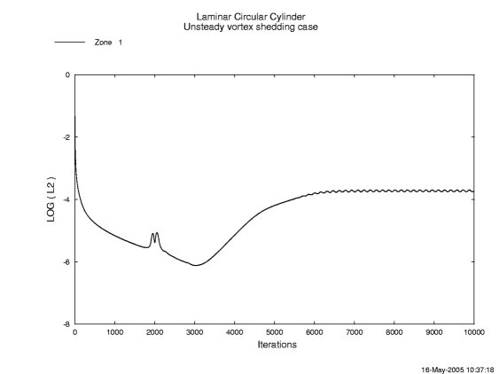
Figure 3. L2 Residual for Case A which used the first order implicit operator.
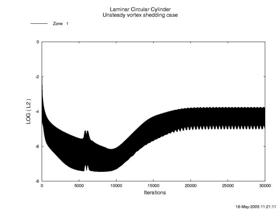
Figure 4. L2 Residual for Case C which used first order implicit and the Global Newton time stepping.
One desired quantity for comparison with the literature is the average total drag coefficient. This was computed by summing the pressure drag and viscous drag coefficient values written to the .lis files as specified by the LOADS keyword block in the Wind-US input .dat files. The first step in this process is to write the lift and drag coefficients to GENPLOT formatted files.
resplt < resplt.A.cd.com
resplt < resplt.B.cd.com
resplt < resplt.C.cd.com
resplt < resplt.D.cd.com
The resulting GENPLOT formatted files are named cd.A.gen, cd.B.gen, cd.C.gen, and cd.D.gen. These files contain the pressure drag and viscous drag coefficients as well as the lift coefficient. Since we desire the total drag coefficient, which is the sum of the pressure and viscous drag coefficients, the simple Fortran90 program cdoutput.f90 was written to compute this from each of the four files. The executable is called cdoutput and it is executed for each run in the manner as shown for Run A, below.
cdoutput < cd.A.gen > cdtot.A.gen
The resulting four files are named cdtot.A.gen, cdtot.B.gen, cdtot.C.gen, and cdtot.D.gen. The result from Run D is plotted in Figure 5 using CFPOST as follows.
cfpost < cfpost.cdtot.D.com
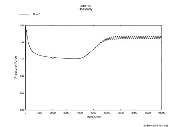
Figure 5. Total drag coefficent for Run D.
The dimensionless frequency, known as the Strouhal number, is given by St = f D/U, where D is the cylinder diameter equal to 1.0 meter and U is the freestream velocity equal to 66.8163 m/s. The parameter f is the frequency of the vortex shedding. To measure this quantity, the velocity and pressure at a point downstream of the cylinder and away from the center of the wake were written to the time history .cth file for each run. It's important to use a point away from the center of the wake because the center of the wake feels the influence of the vortices from both sides (Ref. 2) and will therefore give a value of the frequency double the individual vortex shedding frequency. The x-velocity is read from the time history file and written to a GENPLOT file for each nondimensional time step using the THPLT utility as shown for Run A.
thplt < thplt.A.com
The file u.A.gen results. THPLT can be run in a similar manner for Runs B, C and D, generating the files u.B.gen, u.C.gen and u.D.gen. The x-velocity time history for run A is shown in Figure 6.
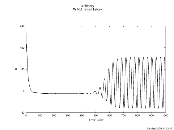
Figure 6. X-velocity history at downstream location x = 1.07 m and y = 0.313 m, Run A.
The easiest way, to compute the frequency is to use the time between peaks of the x-velocity, pressure, or lift coefficent. (The total drag coefficient should not be used to compute the frequency as it feels the influence of both vortices and will give a frequency twice that of the individual vortex shedding frequency.) For Run A, the average nondimensional time between peaks, averaged over the final four peaks, of the x-velocity is 31.0. The time in seconds is t=31.0*Lr/ar, where Lr = 1.0 m and ar = 334.01 m/s, and thus the frequency which is 1/t is equal to 10.777 1/s. The Strouhal number is then computed using the above formula to be 0.161. When the frequency is computed in this manner, the Strouhal number will be referred to as St1. An alternate way of computing the frequency is to use a Fast Fourier Transform (FFT),4 of the velocity data over a given number of iterations. One may write a program to do this, or use mathematical software such as MATLAB5. When using MATLAB to compute the frequency, using the last 2000 points and the last 3000 points, the respective Strouhal numbers, St2 and St3, are 0.150 and 0.1667 for Run A.
In Figure 6, the total drag coeffient is plotted for all four runs using CFPOST.
cfpost < cfpost.cdtotall.com
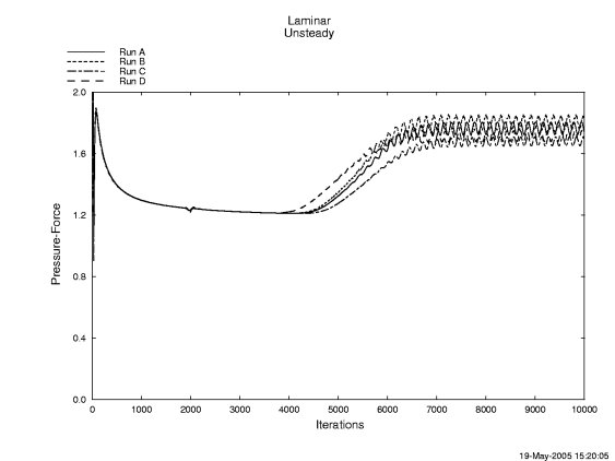
Figure 7. Total drag coefficent for all four runs.
The program cdoutput, used above to compute the total drag coefficient, also computes the average drag coefficient over the last 8000 iterations. This value is listed in the last line of each GENPLOT output file above and is also tabulated in Table 4. The experimental value is 1.78.3 Table 4 also gives the Strouhal numbers computed using the three methods described in the previous section where St1 is the value obtained by hand-calculations of the frequency using the average time between the last four peaks, St2 is the value obtained using an FFT over the last 2000 iterations to compute the frequency, and St3 is the value obtained using an FFT over the last 3000 iterations. The experimental value of the Strouhal number ranges from 0.179 - 0.182.1
| Run | Avg CD | St1 | St2 | St3 |
|---|---|---|---|---|
| A | 1.767 | 0.161 | 0.150 | 0.167 |
| B | 1.804 | 0.164 | 0.175 | 0.167 |
| C | 1.679 | 0.177 | 0.175 | 0.183 |
| D | 1.715 | 0.180 | 0.175 | 0.183 |
As described above, this study compared the use of the first order versus the second order operator in the block implicit method, with and without the Global Newton iteration scheme.
Wind-US version 1.123 was run on an HP xw6200 workstation running the LINUX operating system. The cpu time per iteration and the overall time to compute each case, as reported in the output list files, is given in Table 5.
| Run | CPU time(iter-node) | Total CPU time |
|---|---|---|
| A | 16.93 microsec | 13646 sec |
| B | 16.97 microsec | 13678 sec |
| C | 12.99 microsec | 31415 sec |
| D | 17.23 microsec | 41663 sec |
These cases were originally run by Chris Nelson, Senior Scientist, Innovative Technology Applications Company, LLC, who provided all of his grid, input and output files, as well as valuable insights, so that this validation case could be composed. The cases were re-run, with minor modifications, by Julianne C. Dudek, at NASA Glenn, who composed this web page.
1. Nichols, R. H., and Heikkinen, B. D., "Validation of Implicit Algorithms for Unsteady Flows Including Moving and Deforming Grids," AIAA Paper 2005-0683, 2005.
2. Roshko, A., "On the Development of Turbulent Wakes from Vortex Streets," NACA Report 1191, 1954.
3. Schlicting, H., Boundary-Layer Theory, Sixth Edition, p 17, McGraw-Hill Book Company, 1968.
4. Numerical Recipes in FORTRAN 77: The Art of Scientific Computing,, (ISBN 0-521-43064-X), Copyright 1986-1992 by Cambridge University Press.
5. MATLAB, Copyright 1984-2002, Mathworks, Inc.
This case was created on June 6, 2005 by Chris Nelson, who may be contacted at:
Innovative Technology Applications Company, LLC
Phone: (425) 778-7853
e-mail: Chris Nelson
and Julianne C. Dudek, who may be contacted at:
NASA John H. Glenn Research Center, MS 86-7
21000 Brookpark Road
Brook Park, Ohio 44135
Phone: (216) 433-8513
e-mail: Julianne.C.Dudek@nasa.gov