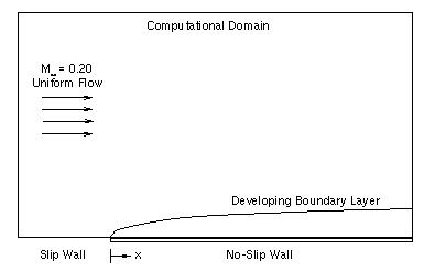
Figure 1: Schematic of Computational Domain.
Figure 1: Schematic of Computational Domain.
The flow being modeled is the incompressible flow over a smooth flat plate originally reported by Wieghardt and later included in the 1968 AFOSR-IFP Stanford Conference on turbulent flows.
This study evaluates the accuracy of the NPARC Chien k-epsilon, WIND Chien k-epsilon, and WIND SST turbulence models and their sensitivity to the near-wall grid spacing.
All of the archive files of this validation case are available in the Unix compressed tar file flpl.tar.Z. The files can then be accessed by the commands
uncompress flpl.tar.Z
tar -xvof flpl.tar
A Cartesian mesh with 111 points in the axial direction and 81 points normal to the viscous wall was used to model this flow. The grid was packed in the streamwise direction to resolve flow gradients near the leading edge of the plate and normal to the plate to resolve the boundary layer.
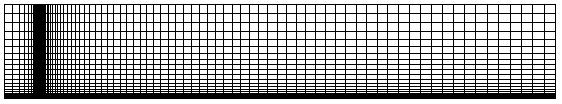
Figure 2: Computational Mesh.
Calculations were made on a series of grids having y+ values of 1, 2, 5, 10, and 30 at the first point off the wall. The figure below shows that these values are representative of the maximum grid spacing along the plate as computed from the WIND Chien k-epsilon solutions.
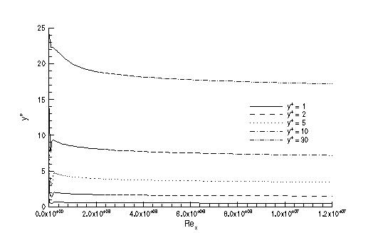
Figure 3: Near-Wall Grid Spacing.
The table below lists the Plot3d files (two-dimensional, multiple-grid, unformatted, whole) and corresponding common grid files used in this study.
| y+ | Plot3D | Common Grid |
| 1 2 5 10 30 |
yp01.x yp02.x yp05.x yp10.x yp30.x |
yp01.cgd yp02.cgd yp05.cgd yp10.cgd yp30.cgd |
The initial (freestream) conditions were generated by WIND at startup. The Chien k-epsilon model was initialized from the existing solution and turbulent viscosity of the SST model after 1000 iterations.
The first 14 grid points upstream of the leading edge of the flat plate were treated as an inviscid wall to provide a uniform profile at the leading edge location while the plate itself was modeled using a viscous wall. The inflow and far-field boundaries were treated as inflow/outflow, and the downstream boundary was specified as a confined outflow. These commands are summarized in the GMAN journal file. The boundary conditions have already been set in the common grid files listed in the Grid section above.
The computation is performed using the time-marching capabilities of WIND to march to a steady-state (time asymptotic) solution. Local time stepping is used at each iteration. The time-marching is performed until the convergence criteria is achieved. For these cases, the solution was monitored every 100 iterations to check for changes in computed skin friction, as well as velocity and turbulent kinetic energy profiles at the last streamwise location for data comparison (Rex=1.03x10⁷).
For the NPARC cacluations, the Baldwin-Lomax model is used for the first 1000 iterations. At that time, the Chien k-epsilon model is initialized from the existing turbulent viscosity. As the solution nears completion, the artificial dissipation is gradually turned off. This artificial dissipation significantly affects the computed skin friction.
The input data file for WIND is flpl.dat.
The WIND flow solver is run, creating the following output files:
| Chien k-epsilon |
Menter SST |
|||||
| y+ | Num. of Iterations |
solution file |
output file |
Num. of Iterations |
solution file |
output file |
| 1 2 5 10 30 |
2500 |
wke01.cfl wke02.cfl wke05.cfl wke10.cfl wke30.cfl |
wke01.lis wke02.lis wke05.lis wke10.lis wke30.lis |
2500 2500 2500 2000 2000 |
wsst01.cfl wsst02.cfl wsst05.cfl wsst10.cfl wsst30.cfl |
wsst01.lis wsst02.lis wsst05.lis wsst10.lis wsst30.lis |
Note that the Chien k-epsilon solutions were initialized from the corresponding Menter SST solutions at 1000 iterations. Thus, the k-epsilon model was run 1500 iterations after initialization.
Convergence information can be obtained from the WIND output files listed below by using the resplt utility program.
| y+ | k-epsilon | SST |
| 1 2 5 10 30 |
wke01.lis wke02.lis wke05.lis wke10.lis wke30.lis |
wsst01.lis wsst02.lis wsst05.lis wsst10.lis wsst30.lis |
Since this study compares both NPARC and WIND results, a common post processor (flplpost.f) was used. This program reads the solution from an NPARC restart file, which means that the WIND solutions must be converted prior to running it.
The figure below shows the computed skin friction using both codes. The grid sensitivity studies shown for the NPARC and WIND Chien k-epsilon models indicate that grid indepenence is obtained using the y+=2 grid. The sensitivity study for the WIND SST model also shows grid independence using the y+=2 grid. While the WIND skin friction results for larger y+ values appear to be much less sensitive than the NPARC results, analysis of the turbulence quantities in the near-wall region reveal that the model predictions begin to break down severely as the mesh spacing exceeds y+=5. The last subfigure compares the skin friction predictions of all three models using the y+=1 grid.
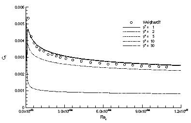
Figure 4a: NPARC Chien k-epsilon Grid Sensitivity Study.
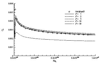
Figure 4b: WIND Chien k-epsilon Grid Sensitivity Study.
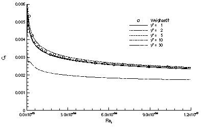
Figure 4c: WIND SST Chien k-epsilon Grid Sensitivty Study.

Figure 4d: Comparison of Grid Independent Solutions.
A comparison of the predicted velocity profiles at several axial locations is given in the figure below.
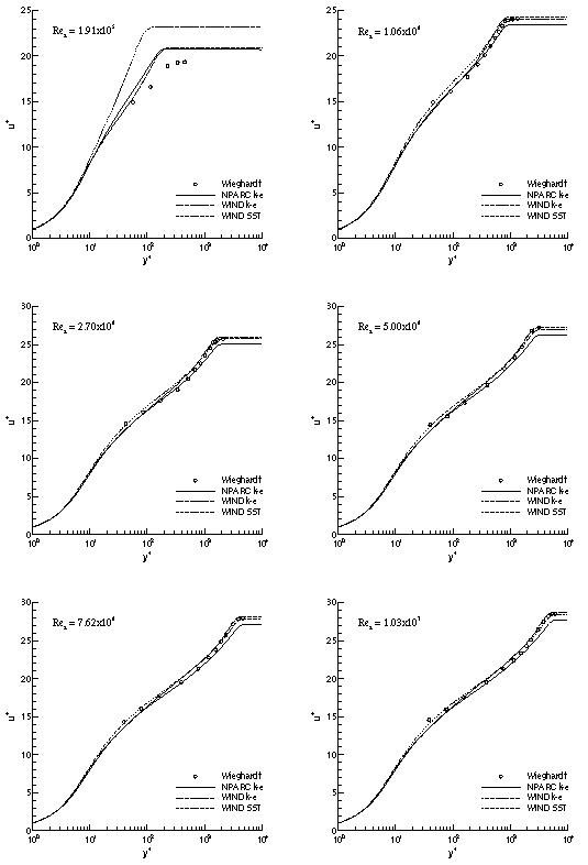
Figure 5: Velocity Profiles Along Flat Plate Using y+=1 Grid.
Examination of the turbulence quantities at the last velocity station is given in the following figures. The first compares the turbulent kinetic energy with the "average" experimental data assembled by Patel, Rodi, and Scheuerer. While neither code matches this data exactly, the WIND results more closely match those obtained by Patel using the Chien model in a 2d boundary layer code. The SST model fails to capture the peak in turbulent kinetic energy due to the form of the k-omega model used in the near-wall region.
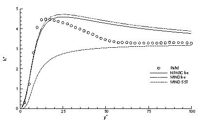
Figure 6: Turbulent Kinetic Energy Profiles in Near-Wall Region.
The turbulent dissipation rate of the Chien models is shown in the next figure. Both models provide reasonable agreement with the assymtotic solution away from the wall.
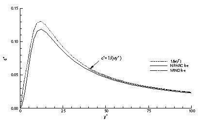
Figure 7: Turbulent Dissipation Rate in Near-Wall Region.
Lastly, the turbulent shear stress is shown below. From this figure, one can observe that the WIND Chien k-epsilon and Menter SST models more closely match the assymptotic solution away from the wall than does the NPARC Chien k-epsilon solution.
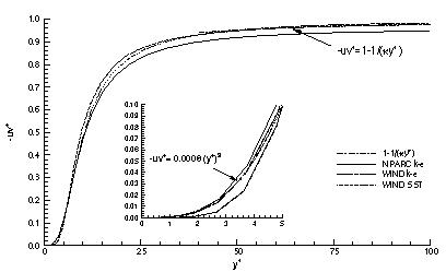
Figure 8: Reynolds Stress in Near-Wall Region.
Coles, D.E., and Hirst, E.A., editors, Computation of Turbulent Boundary Layers - 1968 AFOSR-IFP-Stanford Conference, Vol. 2, Stanford University, CA, 1969.
Patel, V.C., Rodi, W., and Scheuerer, G., "Turbulence Models for Near-Wall and Low-Reynolds Number Flows: A Review," AIAA Journal, Vol. 23, No. 9, Sept. 1985, pp. 1308-1319.
Wieghardt, K. and Tillman, W., "On the Turbulent Friction Layer for Rising Pressure," NACA TM-1314, 1951. [PDF]
Yoder, Dennis A., and Georgiadis, Nicholas J., "Implementation and Validation of the Chien k-epsilon Turbulence Model in the WIND Navier-Stokes Code," AIAA Paper 99-0745, Jan. 1999.
This case was created on November 17, 1998 by Dennis A. Yoder, who may be contacted at
NASA Glenn Research Center, MS 86-7
21000 Brookpark Road
Cleveland, Ohio 44111
Phone: (216) 433-8716
e-mail: Dennis.A.Yoder@lerc.nasa.gov