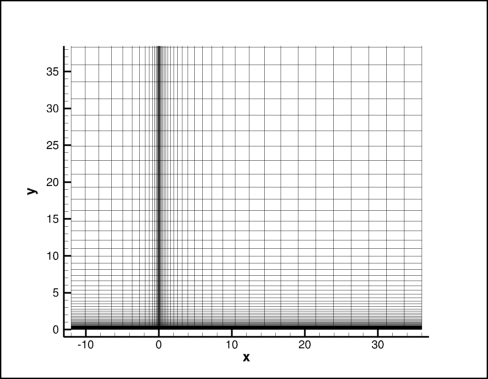
Figure 1. 2-D, structured Mach 4.5 flat plate grid.
In this case, a turbulent boundary layer is developed from a Mach 4.5 flow over a flow plate. The flow conditions are given in Table 1. The Wind-US simulations used several grids and turbulence models. The Wind-US simulations were compared with experimental data from Coles1-3. The skin friction and boundary layer data are available in Table 2. are compared to computational silumations from Wind-US. Typically, the boundary layer along a smooth, flat plate will transition from laminar to turbulent. It is well known that most CFD codes are unable to predict this transition accurately. The Wind-US solutions are fully turbulent flow, e.g. the boundary layer is solely turbulent and does not transition from laminar to turbulent. The available experimental data includes results for several methods of tripping the boundary layer to turbulent earlier than what would naturally occur.
| Mach | Pressure (psia) | Temperature (deg R) | Angle-of-Attack (deg) | Angle-of-Sideslip (deg) |
|---|---|---|---|---|
| 4.512 | 0.0974246 | 108.841 | 0.0 | 0.0 |
| Skin Friction Data | FP4p5_ExpCf.dat |
| Boundary Layer Data | FP4p5_ExpBL.dat |
A TAR file containing all the files (grids, solutions, results) for cases presented here is available for download. To unpack the files, use the command:
tar -xzvf FP4p5.tz
| Wind-US 3.162 |
|---|
| FP4p5.tz |
A 2-D, structured grid was created; it is pictured in Figure 1. The grid consisted of 46 points in the streamwise (x-) direction and 81 points in the transverse (y-) direction. In the streamwise direction, the grid was packed at x=0, the beginning of the flat plate. In the transverse direction, the grid was packed to a nominal spacing of y+=1.0 along the lower boundary, to ensure that the boundary layer was sufficiently resolved. The viscous wall portion of the grid was 36 inches long.
Figure 1. 2-D, structured Mach 4.5 flat plate grid.
The 3-D, structured grid was created by extruding the 2-D, structured grid one cell, 12 inches wide, in the normal (z-) direction. The 3-D, structured grid is shown in Figure 2. The 3-D structured grid was saved in the unstructured format, to be run with the Wind-US unstructured solver.
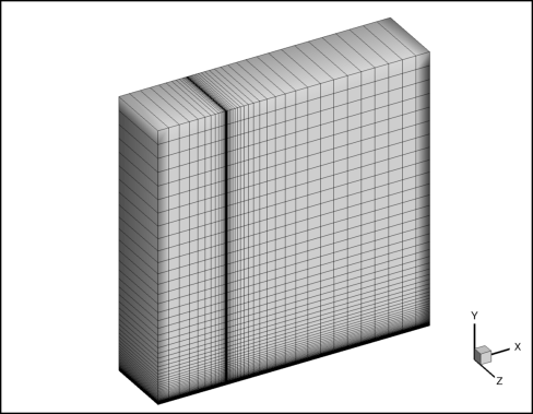
Figure 2. 3-D, structured Mach 4.5 flat plate grid.
A 3-D, unstructured grid was created using the same boundary spacing as the 2-D and 3-D, structured grids. The unstructured grid kept the quadrilateral prism boundary layer from the structured grid. Triangular prisms were used to fill in the remainder of the flow domain. The grid was clustered at x=0 and x=21.5 (the location of the boundary layer probe). The unstructured grid had a total of 12,808 cells.
Along the lower boundary, the 14 points upstream of x=0 were inviscid and the 31 points downstream of x=0 were viscous.

Figure 3. 3-D, unstructured Mach 4.5 flat plate grid.
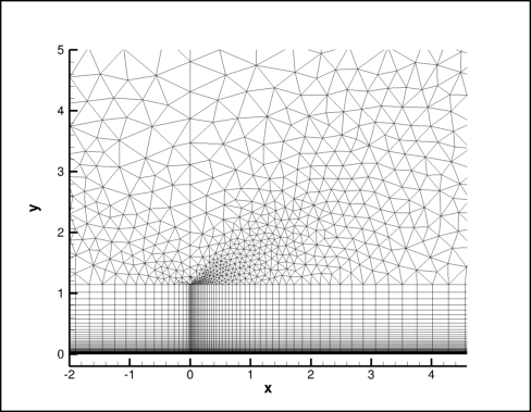
Figure 4. 3-D, unstructured Mach 4.5 flat plate grid; zoom of leading edge.
After creating the unstructured grids, CFPART was used to create lines in the grid to enable the most efficient use of the unstructured line solver. The grid files and CFPART input files are included in Table 4.
| Description | Gridgen File | GMAN Script | CFPART Script | CGD Grid File |
|---|---|---|---|---|
| 2-D, Structured Grid, Structured Solver | FP4p5_StrStr.gg | N/A | N/A | FP4p5_StrStr.cgd |
| 3-D, Structured Grid, Unstructured Solver | FP4p5_StrUns.gg | N/A | FP4p5_StrUns.cfpart.inp | FP4p5_StrUns.cgd |
| 3-D, Unstructured Grid, Unstructured Solver | FP4p5_UnsUns.gg | FP4p5_UnsUns.gman.com | FP4p5_UnsUns.cfpart.inp | FP4p5_UnsUns.cgd |
Boundary conditions for this flat plate case are as shown in Figure 5. Note that the first 14 points along the bottom are set to inviscid, such that the leading edge of the plate is at grid point 15 in the streamwise direction along the bottom of the grid. Although only boundary conditions for the 2-D, structured grid are shown, the boundary conditions are the same for the other grids. For the 3-D grids, the inviscid wall boundary condition is applied to the sidewalls (i.e., z=constant).
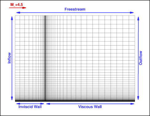
Figure 5. Boundary conditions, shown for the 2-D, structured grid.
Convergence was determined by monitoring the residuals and two flow field quantities key to this case: the wall skin friction coefficient and the u-component of velocity at x=21.5 inches. The algorithm settings used in the DAT file for these unstructured solver cases are listed in Table 5. Note that settings for the structured solver (i.e., choice of RHS method) were different.
| Field | Str-Str SST | Str-Str SST, w/Comp Corr, Press Dilat Off | Str-Str S-A | Str-Uns SST | Str-Uns SST, w/Comp Corr, Press Dilat Off | Str-Uns S-A | Uns-Uns SST | Uns-Uns S-A |
|---|---|---|---|---|---|---|---|---|
| Version | Wind-US 3.162 | Wind-US 3.162 | Wind-US 3.162 | Wind-US 3.162 | Wind-US 3.162 | Wind-US 3.162 | Wind-US 3.162 | Wind-US 3.162 |
| Grid | 2-D, Structured | 2-D, Structured | 2-D, Structured | 3-D, Structured | 3-D, Structured | 3-D, Structured | 3-D, Unstructured | 3-D, Unstructured |
| Solver | Structured | Structured | Structured | Unstructured | Unstructured | Unstructured | Unstructured | Unstructured |
| Iterations | 5,000 | 5,000 | 5,000 | 5,000 | 5,000 | 5,000 | 5,000 | 5,000 |
| Convergence Order | 13 | 13 | 13 | 13 | 13 | 13 | 13 | 13 |
| Method | Default | Default | Default | IMPLICIT UGAUSS LINE EXACT_LHS VISCOUS JACOBIAN FULL CONVERGE FREQUENCY 11 SUBITERATIONS 6 | IMPLICIT UGAUSS LINE EXACT_LHS VISCOUS JACOBIAN FULL CONVERGE FREQUENCY 11 SUBITERATIONS 6 | IMPLICIT UGAUSS LINE EXACT_LHS VISCOUS JACOBIAN FULL CONVERGE FREQUENCY 11 SUBITERATIONS 6 | IMPLICIT UGAUSS LINE EXACT_LHS VISCOUS JACOBIAN FULL CONVERGE FREQUENCY 11 SUBITERATIONS 6 | IMPLICIT UGAUSS LINE EXACT_LHS VISCOUS JACOBIAN FULL CONVERGE FREQUENCY 11 SUBITERATIONS 6 |
| CFL | 1.0 | 1.0 | 1.0 | AUTO DECREASE 2 CFLMAX 200 | AUTO DECREASE 2 CFLMAX 200 | AUTO DECREASE 2 CFLMAX 200 | AUTO DECREASE 2 CFLMAX 200 | AUTO DECREASE 2 CFLMAX 200 |
| Limiters | Default | Default | Default | DQ LIMITER ON RELAX 0.5 | DQ LIMITER ON RELAX 0.5 | DQ LIMITER ON RELAX 0.5 | DQ LIMITER ON RELAX 0.5 | DQ LIMITER ON RELAX 0.5 |
| Dissipation | Default | Default | Default | TVD BARTH 3.0 | TVD BARTH 3.0 | TVD BARTH 3.0 | TVD BARTH 3.0 | TVD BARTH 3.0 |
| Boundaries | IMPLICIT BOUNDARY ON | IMPLICIT BOUNDARY ON | IMPLICIT BOUNDARY ON | IMPLICIT BOUNDARY ON | IMPLICIT BOUNDARY ON | IMPLICIT BOUNDARY ON | IMPLICIT BOUNDARY ON | IMPLICIT BOUNDARY ON |
| RHS | Default | Default | Default | HLLE SECOND, VISCOUS FULL | HLLE SECOND, VISCOUS FULL | HLLE SECOND, VISCOUS FULL | HLLE SECOND, VISCOUS FULL | HLLE SECOND, VISCOUS FULL |
| Gradients | Default | Default | Default | LEAST_SQUARES | LEAST_SQUARES | LEAST_SQUARES | LEAST_SQUARES | LEAST_SQUARES |
| Turbulence Model | SST | SST | SPALART | SST | SST | SPALART | SST | SPALART |
| Turbulence Corrections | none | COMPRESSIBLE, PRESSURE DILATATION OFF | none | none | COMPRESSIBLE, PRESSURE DILATATION OFF | none | none | none |
The options from Table 5 were incorporated into the DAT input files. The input files for the standard SST turbulence model cases listed above are found in Table 6. The other turbulence model options (i.e., Spalart-Allmaras, SST with compressibility correction) are included, but are commented out.
| Case | DAT File |
|---|---|
| Str-Str SST | FP4p5_StrStr.dat |
| Str-Uns SST | FP4p5_StrUns.dat |
| Uns-Uns SST | FP4p5_UnsUns.dat |
Several flow quantities were computed for each case: streamwise (u-) and transverse (v-) velocity; wall skin friction; boundary layer thickness, momentum thickness, and displacement thickness; and Reynolds number. Post-processing scripts were created to compute each of these flow quantities. Table 7 includes the CFPOST scripts used to extract and compute some of these flow quantities.
| Case | CFPOST Script | Full Post-Processing Script |
|---|---|---|
| Str-Str SST | FP4p5_StrStr.cfpost.com | FP4p5_StrStr.pp.csh |
| Str-Uns SST | FP4p5_StrUns.cfpost.com | FP4p5_StrUns.pp.csh |
| Uns-Uns SST | FP4p5_UnsUns.cfpost.com | FP4p5_UnsUns.pp.csh |
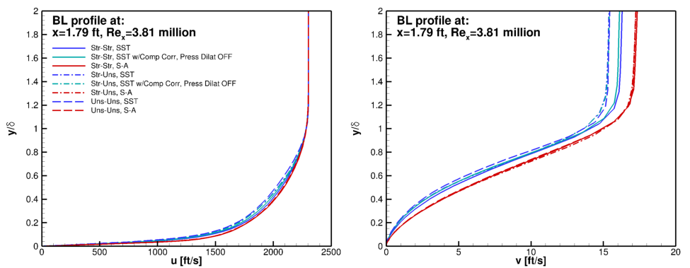
Figure 6. Plots of streamwise (u-) velocity and transverse (v-) velocity through the boundary layer.
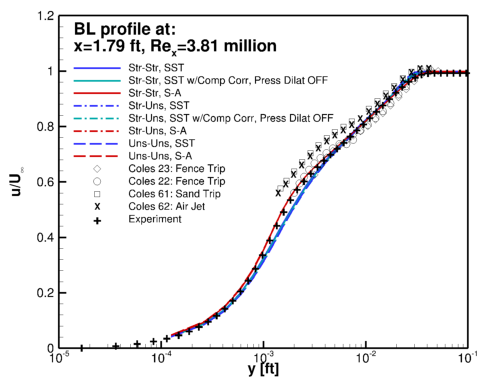
Figure 7. Plot of streamwise (u-) velocity compared to Coles experimental data1-3.

Figure 8. Plots of skin friction and integrated boundary layer thickness.
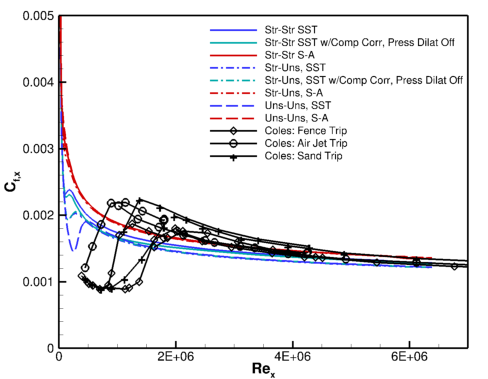
Figure 9. Plots of skin friction compared to Coles experimental data1-3.
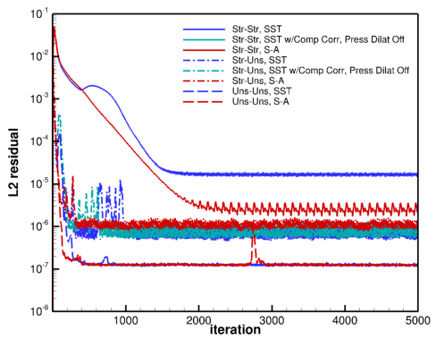
Figure 10. Plot of L2 residuals for determining convergence.
This validation test case was performed by Vance Dippold and Keven Lenahan. Contact: Vance Dippold, MS 5-12, NASA Glenn Research Center, 21000 Brook Park Road, Cleveland, Ohio, 44135.