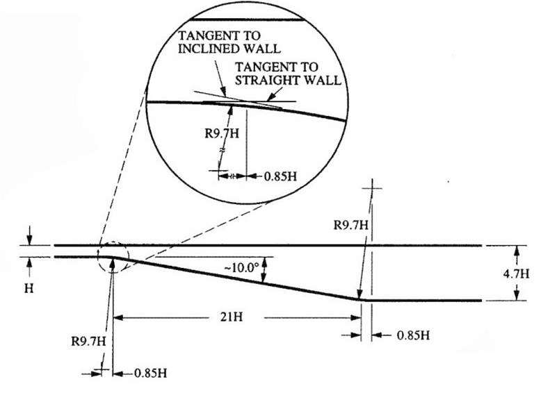
Figure 1: Schematic of Buice-Eaton diffuser [1].
Buice-Eaton
2D Diffuser:
Wind Wall
Function Validation Study
This study examines the performance of the wall functions and turbulence models within the Wind code using the Buice-Eaton diffuser [1]. The Buice-Eaton diffuser, illustrated in Figure 1, is an asymmetric 2D diffuser in which incompressible, fully developed turbulent flow undergoes smooth wall separation and reattachment. The lower wall of the diffuser slopes down at 10° and opens the diffuser up to 4.7 times the entrance height, H=0.59055 in. The flow into the diffuser is approximately Mach 0.058. A total of ten cases were run with the Buice-Eaton diffuser, using y+ values at the wall of 1, 15, 30 and 60, the Menter SST and the Chien K-epsilon turbulence models, and wall functions enabled and disabled. Table 1 details the parameters of each of the ten cases. The solutions from the computational study were compared to axial velocity profile and skin friction data obtained experimentally by Buice and Eaton [1].
Figure
1: Schematic of Buice-Eaton diffuser [1].
|
Analysis |
1 |
2 |
3 |
4 |
5 |
6 |
7 |
8 |
9 |
10 |
|
y+=1 grid |
X |
X |
|
|
|
|
|
|
|
|
|
y+=15 grid |
|
|
X |
X |
|
|
|
|
|
|
|
y+=30 grid |
|
|
|
|
X |
X |
X |
X |
|
|
|
y+=60 grid |
|
|
|
|
|
|
|
|
X |
X |
|
Wall Functions |
|
|
|
X |
|
X |
|
X |
|
X |
|
SST |
X |
|
X |
X |
X |
X |
|
|
X |
X |
|
K-Epsilon, Var Cmu Off |
|
X |
|
|
|
|
X |
X |
|
|
Some files from this study are provided below. Use gunzip to uncompress each archive and tar -xvf to extract the files from archives.
|
File |
Description |
|
Grids files used in study. | |
|
Case 1 files (.dat, .cgd, .cfl, .lis, .tda). |
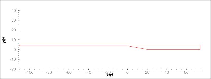
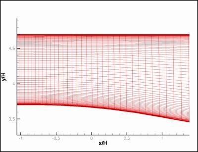
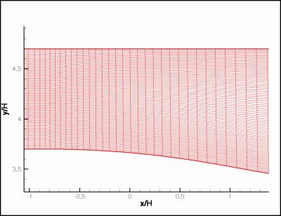
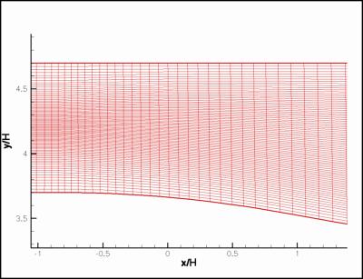
The computational domain, illustrated in Figure 2, extends approximately 65*H upstream and 44*H downstream of the diffuser entrance. From previous studies (link to T.B. validation study), it was determined that a long entrance into the diffuser was necessary to produce the fully developed turbulent flow at the diffuser entrance. Four grids were created to have second grid point y+ values of 1, 15, 30, and 60 at the diffuser entrance. The corresponding second grid point spacing was determined using computational data from a previous study with sufficient near-wall resolution (link). Each grid had 341 points across the axial direction and 81 points in the vertical direct. Figures 3-6 show each grid at the diffuser entrance. Figure 7 shows the computed second grid point y+ values along the lower the lower surface of the diffuser.
Figure
2: Buice-Eaton diffuser computational domain.
Figure
3: Buice-Eaton diffuser y+=1 grid.
Figure
4: Buice-Eaton diffuser y+=15 grid.
Figure
5: Buice-Eaton diffuser y+=30 grid.
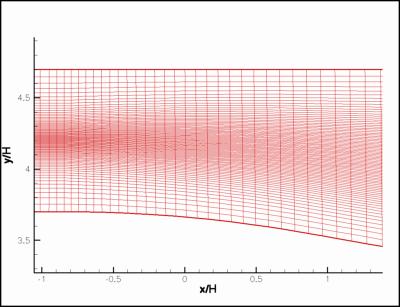
Figure
6: Buice-Eaton diffuser y+=60 grid.
Figure
7: Second grid point y+ values along lower surface
of Buice-Eaton diffuser.
For the Buice-Eaton diffuser, the upper and lower walls are set as “viscous walls.” The inflow boundary was set as an “arbitrary inflow” with uniform conditions prescribed as Mach 0.058142, a 14.7 psi total pressure, and a 530º R total temperature. The “hold_totals” within Wind option was used when specifying the inflow boundary conditions. The outflow boundary was set as the “freestream” boundary condition. The freestream was specified as Mach 0.01, a 14.65 psi static pressure, and a 530º R static temperature. The turbulence models and use of wall functions for each case were specified in accordance to Table 1.
Version 5.0 of the Wind code was used throughout this study. Each case was run with a CFL number of 5. One level of grid sequencing was used to help speed up the convergence of the solution (1-1-0 within Wind). Analyses were performed on two computer systems: an Intel Xeon-based workstation running Linux, and a SGI Origin3400 system.
The convergence of each analysis based upon the convergence of properties along profiles at two separate axial stations in the diffuser. The u and v velocity components, turbulent kinetic energy, and turbulent viscosity profiles at each station were monitored until the solution did not change over the course of several hundred iterations. Typically, the solutions converged with 40,000 iterations at the 1-1-0 grid sequenced level and 40,000 to 80,000 iterations at the 0-0-0 grid sequenced level. However, several cases required up to 150,000 iterations at the 0-0-0 grid level.
CFPOST uses the freestream velocity to compute the skin friction, Cf. Because the diffuser is enclosed, there is no “freestream.” Therefore a better procedure was needed to calculate the skin friction. A Matlab script was written to compute the bulk velocity, Ubulk across the entrance of the computational domain. The bulk velocity was computed from:

in which n is the number of points vertically across the diffuser (81 for the grids used in this study). Therefore, the skin friction for each point along the lower wall was computed from:

in which ρ is the density. Similarly, the skin friction along the upper wall was computer from:

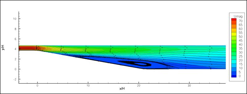
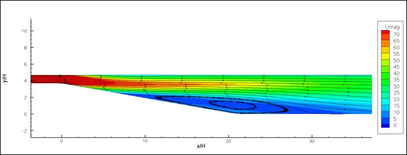
The experimental results show that separation occurred at 5.5*H downstream of the entrance into the diffuser, where H is the height of the diffuser at the entrance. Reattachment took place at 29.2*H. Figures 8-11 show the skin friction along the lower and upper walls of the diffuser for the turbulence model and wall function comparisons. Both y+=1 grid cases (Cases 1 and 2) predicted separation earlier than what was seen in the experiment. However, there is pretty good agreement between several SST model cases (Cases 1, 3, 4, 5, 6) for where the flow reattaches in the diffuser, roughly 29.5*H. For SST cases, only the two y+=60 cases (Cases 9, 10) differ at reattachment, and Case 10 (without wall functions) fails to predict separation. It should be noted that the K-epsilon model gives a very liberal prediction for flow reattachment on the lower wall of the diffuser. Furthermore, the K-epsilon model predicts flow separation of the upper wall of the diffuser, which is not observed in the experimental data. Plots of the velocity contours and streamlines for the SST and K-epsilon models are shown in Figures 12-13. Figures 14-15 show plots of the TKE contours as predicted by the SST and K-epsilon models. The normalized velocity profiles through the diffuser are plotted in Figures 16-17, and again show significant disagreement between the SST and K-epsilon turbulence models. The diffuser velocity profiles plotted in Figure 17 show that the SST model matches the data well (outside of the early separation on the lower surface) even up to the y+=30 grid, with and without wall functions. The SST y+=60 grid is clearly beyond the usefulness of wall functions for this flow.
Figure
8: Skin friction along lower wall of Buice-Eaton diffuser, turbulence
model comparison.
Figure
9: Skin friction along upper wall of Buice-Eaton diffuser, turbulence
model comparison.
Figure
10: Skin friction along lower wall of Buice-Eaton diffuser, wall
function comparison.
Figure
11: Skin friction along lower wall of Buice-Eaton diffuser, wall
function comparison.
Figure
12: Velocity contours and streamlines for Case 1: SST turbulence
model, y+=1.
Figure
13: Velocity contours and streamlines for Case 2: K-epsilon
turbulence model, y+=1.
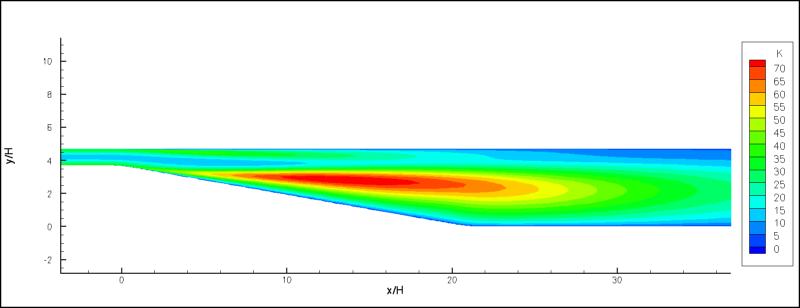
Figure
14: TKE contours and streamlines for Case 1: SST turbulence
model, y+=1.
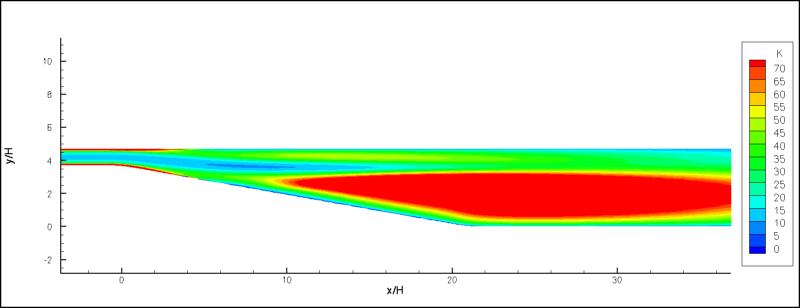
Figure
15: TKE contours and streamlines for Case 2: K-epsilon
turbulence model, y+=1.
Figure
16: Velocity profiles in Buice-Eaton diffuser. Comparison of
turbulence models.
Figure
17: Velocity profiles in Buice-Eaton diffuser. Comparison of wall
function/wall integration cases.
From this set of parametric studies on the Buice-Eaton diffuser, a couple of conclusions can be made. First, the SST turbulence model does a much better job of predicting the flow in this diffuser than the Chien K-epsilon turbulence model. The only fault is that the SST model gives a more conservative prediction for when separation occurs. Next, Wind’s wall functions (paired with the SST turbulence model) are not a good choice for separated flow: flow separation is delayed on the y+=30 grid and results are poor on the y+=60 grid.
[1] Buice, C. U. and Eaton, J. K., “Experimental Investigation of Flow Through an Asymmetric Plane Diffuser,” J. Fluids Engineering, Vol. 122, June 2000, pp. 433-435.
This study was performed on March 16, 2003 by Vance Dippold, III who my be contacted at:
NASA Glenn Research Center
21000 Brookpark Road, M.S.
86-7
Cleveland, OH 44135
Phone: (216) 433-8365
e-mail:
Vance.F.Dippold@nasa.gov