
This section is intended primarily for new users to demonstrate the simulation process using Wind-US. More experienced users may find this section useful as a road map through the simulation process and to help demonstrate new features. The approaches presented here are by no means unique, and detailed information is excluded by design. The user is referred to later sections of this User's Guide for more detailed information on the various aspects of running Wind-US, and in particular to the Keyword Reference section for more in-depth discussions on the choices available for each input keyword.
The approach taken here is to discuss the flow simulation process using as an example a simple subsonic internal flow in a diverging duct. The various files and scripts used in this tutorial may be obtained by following the instructions in the Downloading Files section.
While it is clearly impossible to demonstrate every option in Wind-US with a single application, the basic mechanics of using Wind-US are demonstrated with this case. Additional abbreviated examples are also provided in the Keyword Reference section for specific keywords. For details of the flow simulation process for more complex cases, please see the various example applications accessible from the Wind-US Validation home page.
The solution process using any conventional time-marching Navier-Stokes code is basically the same, and may be divided into the following steps:
As for any project, the first step is to gather all of the information required to completely specify the problem to be analyzed. Of course, as the flow simulation process proceeds, missing information will become apparent. The required information can be divided into three major categories - geometry, flow conditions, and boundary conditions. It is also important to understand the ultimate goal of the simulation. For example, is an accurate drag prediction required? Or, is lift required, but only to within 5%? The answers to these types of questions will determine the detail of the input information required to provide the necessary level of detail and accuracy in the solution.
The more geometric details that can be determined for the target application, the more likely the results will provide an accurate simulation of the flow field. This is not to say that all geometric components must be modeled. Resolving fine geometric details of a configuration requires more grid points, and, as a result, longer run times. The level of detail to which the geometry must be modeled depends on the type of results required and the acceptable turn-around time.
The geometry of the Test Case 4 example is shown in the figure below. The duct is 8 inches long, and the entrance and exit heights are 1 inch and 2 inches, respectively.
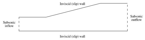
The desired result from this calculation is the pressure distribution along the upper and lower walls, and the mass flow rate to within 10%. Thus, resolving the sharp surface gradients at the corners is not necessary. Other detailed geometric features such as weld joints, for example, are also not modeled. If the fine details of the boundary layer in the vicinity of the joints were important, then a significantly more detailed geometry description would be required.
In addition to the geometric information, flow conditions are also required, and are used to set the reference conditions used in non-dimensionalizing the governing equations solved by Wind-US. As with the geometric information, the simulation results will only be as good as the flow condition information provided by the user. Flow conditions should be specified that are representative of the flow being solved, so that the nondimensional variables used in the code are on the order of 1.0. A good choice is the inlet conditions for internal flows, and the freestream conditions for external flows.
For this example case, the inlet Mach number, total pressure, and total temperature are 0.78, 15 psi, and 600 °R, respectively. Starting from these conditions, the Reynolds number based on the inlet duct height can be computed as 3.023 × 10⁵.
Information is also required at boundaries that are at the "outer edges" of the computational domain. These boundary conditions are used to model the interaction between the flow inside the computational domain and surfaces or flows outside the domain. In fact, the boundary conditions are perhaps the most important factor influencing the accuracy of the flow computation.
Conditions at flow interface boundaries (i.e., boundaries between flows that are inside and outside the computational domain such as inflow, outflow, and freestream boundaries) must be known to the level of accuracy required by the simulation. For example, if flow rates are required to within 0.1%, even slight variations in total pressure at the inflow boundary must be specified. The number of conditions to be specified at a flow interface boundary depends on whether the flow is entering or leaving the computational domain, and whether it is subsonic or supersonic.
Information must also be specified at surface interface boundaries, such as solid walls and bleed regions. Simply specifying the type of boundary, such as an adiabatic no-slip wall, is often sufficient. Additional information may also be required, though, such as the wall temperature. The level of detail that is needed for this information is determined, as discussed above, by the level of detail and accuracy required in the results.
Note that other types of boundaries may be present within the overall computational domain, that are not at the "outer edges." Multi-zone problems will have zonal interface boundaries. Some configurations will also have boundaries resulting from the grid topology, such as self-closing and singular axis boundaries. These types of boundaries need only be labeled.
For Test Case 4 the flow at both the inflow and outflow planes will be subsonic. Three conditions are needed at the inflow boundary, and one is needed at the outflow boundary. At the inflow boundary, uniform flow is specified, with total pressure and temperature equal to the inlet values of 15 psi and 600 °R. Since extreme accuracy in the solution is not needed, constant total conditions at the inflow are sufficient. At the outflow boundary, the exit static pressure is set to 14.13 psi. The Reynolds number for Test Case 4 is large enough that the boundary layers will have little influence on the pressure distribution within the duct. The upper and lower boundaries are therefore specified as inviscid (slip) walls.
The procedure used to set boundary conditions when running Wind-US is discussed later in this tutorial. Additional details on all the boundary conditions available in Wind-US are presented in the Boundary Conditions section.
Wind-US uses externally-generated grids. The grids for all the zones must therefore be created before running Wind-US. The geometry of the application governs the overall shape of the boundaries, but the approach to gridding the flow field is not unique.
The Wind-US flow simulator provides considerable flexibility. Grid lines can conform to complex shapes or may pass through regions not in the flow field. The grid may be divided into zones to conform to the geometry better, to allow grid embedding (i.e., zones with finer grids in regions of high gradients like boundary layers), and/or to allow parallel computation. These zones may be abutting or overlapping, and overlapping grids may be single- or double-fringed.
Wind-US can compute flows using structured or unstructured grids. In this tutorial a structured grid is used. The indices (i, j, k) thus represent a curvilinear coordinate system, and physical Cartesian coordinates (x, y, z) are defined for each integer combination of indices. The handedness of both the physical and curvilinear coordinate systems is required to be the same at all points in the grid, i.e., both must be either left-handed or right-handed. Additionally, at least three grid points must fall between any two grid lines which represent a boundary within the computational domain. For example, if the k = 1 boundary represents a solid surface and an adjacent k boundary represents a symmetry plane, the symmetry plane must be at k = 5 or higher, so that the three points k = 2, 3, and 4 (at least) lie between the two boundaries.
The method used to create the grid is completely up to the user. For complex geometries, a sophisticated grid generation program is normally used. For very simple geometries, it may be easier to write a short program that constructs a grid using algebraic techniques.
The computational grid used by Wind-US for a particular case is stored in a Common Grid (.cgd) file, so named because the file is formatted according to Boeing's Common File Format. [Wind-US also supports the use of CGNS files for the grid and flow solution, using the CGNSBASE keyword. This tutorial, however, uses common files.] The (x, y, z) coordinates of all the grid points, zone coupling information, grid units, and scaling data are stored in this file. [See the Common File User's Guide for details about the internal structure of Common Files.]
Since some grid generation codes do not produce .cgd files directly, a separate utility called cfcnvt is included with Wind-US that may be used to convert a variety of file formats, including PLOT3D files, to Common Files. A typical procedure is thus to first store the grid file as a PLOT3D xyz file, which is an available option in most general-purpose grid generation codes, and then convert it to a .cgd file using cfcnvt.
Zone coupling information is then added to the .cgd file using either the GMAN or MADCAP pre-processing utility. This is typically done at the same time as the boundary condition types are defined, and is discussed in the Define the Input - Boundary Conditions section later in this tutorial. The .cgd file may then be examined to assess grid quality and list information about the points and zones in the grid. GMAN or MADCAP may also be used to generate the interior grid itself, given the grids on the zonal boundaries. Descriptions of these capabilities, and others, may be found in the user's guides for GMAN and MADCAP.
Even when third-party mesh-generation codes are used to create the grid file, GMAN or MADCAP should still be used to perform grid quality checks and confirm that no boundary surface condition remains undefined. Often zone coupling information, particularly for non-point-matched boundaries, is missing from the file.
The computational grid for Test Case 4 was constructed by simple algebraic techniques using the following program, called case4.mesh.f90, which writes a PLOT3D xyz file in 2-D unformatted multi-zone form to case4.xyz, without an iblank array.
         Program mesh

   !-----Purpose:  This subroutine computes a 2-D three-zone grid for a
   !               simple diffuser, one of the test cases supplied with
   !               Wind-US. The grid is written to a file in PLOT3D 2-D
   !               unformatted form, without iblank'ing.

   !-----Called by:

   !-----Calls:

         Implicit none
   !-----Parameter statements
         Integer IDIM,JDIM    ! Max dimensions
         Integer NBLKS        ! Number of blocks
         Parameter (IDIM = 33, JDIM = 11)
         Parameter (NBLKS = 3)
   !-----Local variables:
         Integer i,j          ! Indices in x and y directions
         Integer iblk         ! Current block number
         Integer imax(NBLKS),jmax(NBLKS) ! Block grid sizes
         Real dx(NBLKS),dy(NBLKS)        ! Non-dim grid increments in blks
         Real x(IDIM,JDIM),y(IDIM,JDIM),z(IDIM,JDIM)   ! Grid coordinates
         Real xdiff1,xdiff2   ! x at start/end of diffuser section
         Real xloc            ! Local x coordinate
         Real xmax            ! x at end of duct
         Real xstrt(NBLKS),xend(NBLKS)   ! Non-dim x limits of blocks
         Real ymax            ! Max y at x = xloc
         Real ymax1,ymax2     ! Max y at start/end of diffuser section
         Real yslope          ! Slope of diffuser upper wall
         Real ystrt(NBLKS),yend(NBLKS)   ! Non-dim y limits of blocks

   !-----Define geometric parameters (This mesh is in inches.)

         Data xdiff1,xdiff2,xmax /2.0, 6.0, 8.0/
         Data ymax1,ymax2 /1.0, 2.0/

   !-----Set relative sizes and grid increments for each block

   !-----Block 1
         imax(1) = 17
         jmax(1) =  6
         xstrt(1) = 0.0
         ystrt(1) = 0.0
         xend (1) = 0.5
         yend (1) = 0.5
         dx(1) = (xend(1) - xstrt(1))/(imax(1) - 1)
         dy(1) = (yend(1) - ystrt(1))/(jmax(1) - 1)
   !-----Block 2
         imax(2) = 33
         jmax(2) = 11
         xstrt(2) = 0.0
         ystrt(2) = yend(1)
         xend (2) = xend(1)
         yend (2) = 1.0
         dx(2) = (xend(2) - xstrt(2))/(imax(2) - 1)
         dy(2) = (yend(2) - ystrt(2))/(jmax(2) - 1)
   !-----Block 3
         imax(3) = 17
         jmax(3) = 11
         xstrt(3) = xend(1)
         ystrt(3) = 0.0
         xend (3) = 1.0
         yend (3) = 1.0
         dx(3) = (xend(3) - xstrt(3))/(imax(3) - 1)
         dy(3) = (yend(3) - ystrt(3))/(jmax(3) - 1)

   !-----Open grid file, write header info

         Open (unit=2, file='case4.xyz', form='unformatted')
         Write (2) NBLKS
         Write (2) (imax(iblk),jmax(iblk),iblk=1,NBLKS)

   !-----Construct the grid

         yslope = (ymax2 - ymax1)/(xdiff2 - xdiff1)   ! Slope of diff wall
         Do iblk = 1,NBLKS           ! Loop over no. of blocks
            Do i = 1,imax(iblk)      ! Loop over no. of x points
   !-----------Compute x coordinates
               xloc = (xstrt(iblk) + dx(iblk)*(i-1))*xmax
               Do j = 1,jmax(iblk)   ! Loop over no. of y points
                  x(i,j) = xloc
               End do
   !-----------Get local max y, then compute y coordinates
               If (xloc <= xdiff1) then          ! Upstream of diffuser
                  ymax = ymax1
               Else if (xloc >= xdiff2) then     ! Downstream of diffuser
                  ymax = ymax2
               Else                              ! In diffuser
                  ymax = ymax1 + yslope*(xloc-xdiff1)
               End if
               Do j = 1,jmax(iblk)   ! Loop over no. of y points
                  y(i,j) = (ystrt(iblk) + dy(iblk)*(j-1))*ymax
               End do
            End do

   !-----Write the grid file in PLOT3D xyz format

            Write (2) ((x(i,j),i=1,imax(iblk)),j=1,jmax(iblk)), &
                      ((y(i,j),i=1,imax(iblk)),j=1,jmax(iblk))
         End do
         Stop
         End
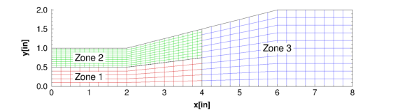
The resulting grid is shown below. Three zones are used, with grid sizes of 17 × 6, 33 × 11, and 17 × 11, respectively. [This geometry is simple enough that a single-zone grid would be sufficient, but a three-zone grid is used for illustrative purposes.]
The grid file written by the above program, named case4.xyz, was converted to a .cgd file named case4.cgd using cfcnvt, as shown in the following runstream. Lines in slanted type were typed by the user.
   cfcnvt
    ****************************************************************************
    * Warning: This software contains technical data whose export is           *
    * restricted by the Arms Export Control Act (Title 22, U.S.C., Sec 2751,   *
    * et seq.) or Executive Order 12470. Violation of these export-control     *
    * laws is subject to severe criminal penalties. Dissemination of this      *
    * software is controlled under DoD Directive 5230.25 and AFI 61-204.       *
    ****************************************************************************
             ******* Common File Convert Utilities ******
    CFCNVT - Version 1.60 (last changed 2014/06/05 17:01:11)

      0: Exit program
      2: Import   a Common File
      3: Compress a Common File
      4: Break Common File into multiple transfer files
      5: Combine multiple transfer files into Common File
      6: Append one Common File to another
      7: Convert Common File binary to a text file
      8: Convert Common File text to a binary file
     11: Convert PLOT3D/Pegsus file to Common File
     12: Convert GASP     file to Common File
     13: Convert OVERFLOW file to Common File
     14: Convert Common File to OVERFLOW file
     15: Convert CFPOST GPU file to Common File GPC
     16: Convert ascii rake to Common File rake CGF
     17: Convert Pegsus 4.0 files to Common File
     18: Convert Common File CFL to Plot3d Q

     Enter the number from one of the above requests
   11

      PLOT3D file type menu

      0: Main menu
      1: Convert a PLOT3D Grid     (.x) file to CFS.
      2: Convert a PLOT3D Solution (.q) file to CFS.
      3: Convert a PLOT3D Function (.f) file to CFS.

     Enter the number from one of the above requests
   1

      PLOT3D Number of Grids menu

      0: Main menu
      1: PLOT3D Single zone format.
      2: PLOT3D Multi  zone format.

     Enter the number from one of the above requests
   2

      PLOT3D Zone dimension menu

      0: Main menu
      1: PLOT3D 2d zone format.
      2: PLOT3D 3d zone format.

     Enter the number from one of the above requests
   1

      PLOT3D Format menu

      0: Main menu
      1: PLOT3D Formatted   (ASCII).
      2: PLOT3D Unformatted (sequential binary).
      3: PLOT3D Binary (c binary).

     Enter the number from one of the above requests
   2

      PLOT3D Iblank menu

      0: Main menu
      1: PLOT3D grid with    IBLANK format.
      2: PLOT3D grid without IBLANK format.

     Enter the number from one of the above requests
   2

      PLOT3D Precision menu

      0: Main menu
      1: PLOT3D Single precision format.
      2: PLOT3D Double precision format.

     Enter the number from one of the above requests
   1

      PLOT3D INTOUT menu

      0: Main menu
      1: No INTOUT/XINTOUT file.
      2: INTOUT file.
      3: XINTOUT file.

     Enter the number from one of the above requests
   1
     Enter PLOT3D .x file to convert with suffix
   case4.xyz
     Enter output Common File name with suffix
   case4.cgd
     zone, idim,jdim,kdim:           1          17           6           1
     zone, idim,jdim,kdim:           2          33          11           1
     zone, idim,jdim,kdim:           3          17          11           1
     imax,jmax,kmax:          33          11           1
     Global maximums set as follows:
     mimax 33
     mjmax 11
     mkmax 1
     mpts: 363
     recl: 726
    Processing zone ZONE   1
    Writing mesh data
     imax,jmax,kmax:          17           6           1
    Processing zone ZONE   2
    Writing mesh data
     imax,jmax,kmax:          33          11           1
    Processing zone ZONE   3
    Writing mesh data
     imax,jmax,kmax:          17          11           1

      0: Exit program
      2: Import   a Common File
      3: Compress a Common File
      4: Break Common File into multiple transfer files
      5: Combine multiple transfer files into Common File
      6: Append one Common File to another
      7: Convert Common File binary to a text file
      8: Convert Common File text to a binary file
     11: Convert PLOT3D/Pegsus file to Common File
     12: Convert GASP     file to Common File
     13: Convert OVERFLOW file to Common File
     14: Convert Common File to OVERFLOW file
     15: Convert CFPOST GPU file to Common File GPC
     16: Convert ascii rake to Common File rake CGF
     17: Convert Pegsus 4.0 files to Common File
     18: Convert Common File CFL to Plot3d Q

     Enter the number from one of the above requests
   0
The next step is to define the input data. Input is required to specify the flow and initial conditions, the boundary conditions, and various parameters controlling the physical and numerical models to be used when running the code.
The primary file controlling how Wind-US is executed is the Input Data (.dat) file. With many CFD codes the input data are specified using Fortran namelist and/or formatted input. With Wind-US, the input is specified using descriptive keywords. The formatting rules for the .dat file are described in the "Files" section.
This section is intended as an introduction to some of the more commonly-used keywords. After reading the information presented here, a new user should supplement it with the detailed information in the Keyword Reference section. For many cases, the default values for the various keyword options are acceptable, but users should become familiar with all of the options for the most effective use of Wind-US.
The first three lines of the file are reserved for geometry, flow condition, and arbitrary titles, respectively. Each of these titles may be up to 64 characters long.
Comment lines, beginning with a / or !, may be placed anywhere in the file after the first three lines. The readability of the .dat file may be improved significantly through the liberal use of comments - for example, to separate logical sections of the data file like boundary conditions, numerical operators, convergence monitoring parameters, etc. Trailing comments are also supported.
Blank lines can also be used to improve the readability of the .dat file.
Long commands may be split across multiple lines. To indicate that the current command continues, the last character on the line must be \.
With most CFD codes, boundary conditions are completely specified in the input data file. With Wind-US, however, setting boundary conditions is a two-step process, defining first the type of boundary, and then any values that are needed.
The first step is to label each boundary of each zone with the type of boundary condition to use, such as "viscous wall," "outflow," or "coupled." This is done using either the GMAN or MADCAP pre-processing code, and the information is stored in the Common Grid (.cgd) file. Details on the boundary condition types available for use with Wind-US are in the Boundary Conditions section.
Boundary condition types may be specified for all or part of a boundary, allowing multiple boundary conditions on a single boundary. "Coupled" zonal interface boundaries do not have to be explicitly labeled by the user. Both GMAN and MADCAP can automatically examine the grid to find them and determine the zones involved, compute the geometric interpolation factors, and store the information in the .cgd file. GMAN or MADCAP is also used to cut holes and generate interpolation coefficients for overlapping ("chimera") boundaries. The process is currently not completely automated for chimera boundaries.
The second step is to define any values needed for a particular boundary condition, such as an exit pressure or a bleed rate. This information is specified in the .dat file. Keywords are available to specify conditions at inflow boundaries (ARBITRARY INFLOW), at outflow boundaries (COMPRESSOR FACE, DOWNSTREAM MACH, DOWNSTREAM PRESSURE, MASS FLOW), along solid walls (MOVING WALL, TTSPEC, WALL TEMPERATURE), in bleed and blowing regions (BLEED, BLOW), and across actuators and screens (ACTUATOR | SCREEN).
The flow conditions (Mach number, and static or total pressure and temperature, plus the angles of attack and sideslip) are specified using the FREESTREAM keyword. These conditions, along with a reference length based on the units used in the .cgd file, are used as the reference conditions and determine the Reynolds number.
The usual procedure with Wind-US is to start a new problem by setting the initial conditions at each grid point equal to the values specified using the FREESTREAM keyword. Other keywords allow different values to be used in different zones (ARBITRARY INFLOW), a boundary layer to be added along a specified surface in a zone (BL_INIT), and reinitialization of the flow in specified zones after a restart (REINITIALIZE). Previously-run, partially-converged cases will normally be restarted using the current solution as initial conditions (RESTART). More information about flowfield initialization may be found in the Geometry and Flow Physics Modeling - Flowfield Initialization section.
Wind-US may be used for three-dimensional, two-dimensional, quasi-three-dimensional, or axisymmetric configurations. Internally, Wind-US treats structured grids as three-dimensional, with indices i, j, and k. Two-dimensional cases simply have kmax = 1, with the i-j grid lying in a non-zero, z-constant plane. The effect of area variation in an otherwise two-dimensional configuration may be modeled using Wind-US's quasi-three-dimensional capability, which is activated by setting the z-coordinate equal to the "width" of the geometry at each grid point. Axisymmetric configurations are modeled using a two-dimensional grid in conjunction with the AXISYMMETRIC keyword. Unstructured grids are only supported for three-dimensional configurations. More details may be found in the Geometry and Flow Physics Modeling - Symmetry Considerations section.
The default equations solved by Wind-US are the full Reynolds-averaged Navier-Stokes (RANS) equations. Keywords are available to solve the Euler equations (TURBULENCE), parabolized Navier-Stokes equations (MARCHING), or the thin-layer Navier-Stokes equations (TSL). See the Numerical Modeling - Thin-Shear-Layer Calculations section for more information about the thin-layer option.
A variety of turbulence models are available in Wind-US through the TURBULENCE keyword. These include algebraic models, one- and two-equation turbulent transport models, non-linear and algebraic Reynolds stress models, and hybrid RANS/LES (large eddy simulation) models. A laminar flow option is also available using the TURBULENCE keyword. Laminar-turbulent transition may be simulated using: specified laminar and turbulent zones, a specified transition region via the TTSPEC keyword, or the Menter shear stress transport (SST) turbulence model with bypass transition prediction. See the Geometry and Flow Physics Modeling - Turbulence Models section for more information.
A variety of gas models are available in Wind-US to complete the equation set. The fluid may be treated as a thermally and calorically perfect gas, a thermally perfect gas (i.e., frozen chemistry), equilibrium air, or a mixture undergoing a finite rate chemical reaction. For a thermally and calorically perfect gas, the values of the ratio of specific heats (γ), the laminar and turbulent Prandtl and Schmidt numbers, and the gas constant may be set using the GAS, PRANDTL, and SCHMIDT keywords. Real gas chemistry models are selected using the CHEMISTRY keyword. Several different chemistry packages are available in the form of files containing thermodynamic data, finite rate coefficients, and transport property data, described in the Files - Chemistry Files section.
In Wind-US, the number of iterations or time steps to perform in a given run is defined in terms of cycles and iterations per cycle. An iteration advances the solution one time step. A cycle consists of a solution pass over all the zones. Zone coupling, the process whereby Wind-US exchanges flowfield information between zones, only occurs at the end of each cycle. The Common Flow (.cfl) file is also updated only at the end of each cycle. The number of cycles to be performed is set using the CYCLES keyword, and the number of iterations per cycle, which may vary from zone to zone, is set using the ITERATIONS keyword. The default is five iterations per cycle.
The time step size is controlled by the CFL# keyword. By default, local time stepping is used, so that the solution advances at a different rate at each grid point. For unsteady problems, of course, the same time step size should be used throughout the flowfield, and an option is available with the CFL# keyword for this purpose. A Runge-Kutta time step formulation may be specified, using the STAGES keyword, and may be used for both steady and unsteady flows. Global Newton iteration, dual time stepping, and second-order time marching are also available using options in the TEMPORAL keyword block.
See the "Numerical Modeling" section for more information about cycles and iterations, and about time step options.
The IMPLICIT keyword allows a variety of implicit operators to be specified, including point Jacobi, Gauss-Seidel, and MacCormack modified approximate factorization. Also available are options to: (1) turn off the implicit operator completely, resulting in an explicit calculation; (2) use a scalar (diagonalized) implicit operator; or (3) use a full block implicit operator. For these last three options, a different implicit operator may be specified for each computational direction.
The default is to use the full block operator in viscous directions, and the scalar (diagonalized) operator in inviscid directions.
The IMPLICIT BOUNDARY keyword may be used to specify that implicit boundary conditions are to be used on "wall" boundaries. This should improve stability when the CFL number is above about 1.3.
Through use of the RHS keyword, a wide variety of explicit operators are available for evaluation of the first-derivative terms on the right-hand side. These include a central difference scheme, the upwind Coakley, Roe, Van Leer, HLLE, HLLC, and Rusanov schemes, and modified versions of the upwind schemes (except Coakley) for stretched grids. Depending on the type of scheme used, the accuracy may be specified as anywhere from first to fifth order. The default is Roe's second-order upwind-biased flux-difference splitting algorithm, modified for stretched grids.
Various smoothing options are available in Wind-US to dampen instabilities that may occur under certain conditions. These include second- and fourth-order explicit smoothing (SMOOTHING, BOUNDARY-DAMP), and total variation diminishing (TVD) flux limiting for some of the explicit operators (TVD, BOUNDARY TVD). More details on the various damping options are in the Numerical Modeling - Explicit Operator section.
The ACCELERATE keyword may be used, in conjunction with the SMOOTHING and CFL# keywords, to increase the time step near the beginning of a calculation, in order to more quickly get through the start-up transients that may occur in the first few hundred iterations.
A grid sequencing capability is also available, using the SEQUENCE keyword, that may help speed convergence. With this option, grid points are removed from selected regions of the flowfield, resulting in a coarse-grid solution which is obtained in a fraction of the time it would have taken for a full-grid solution. At the end of each run, the solution is interpolated back onto the original grid to aid in restarting the solution, and to provide a continuous flowfield for post-processing. The full grid should of course be used when the solution nears convergence.
See the "Numerical Modeling" section for more information about the convergence acceleration and grid sequencing capability.
The convergence criterion, in terms of the required value or reduction of the maximum residual, may be specified using the CONVERGE keyword. Integrated forces, moments, and/or mass flow may also be used to monitor convergence, by using the LOADS keyword to periodically compute and print these values for specified areas of a computational surface.
For unsteady flow problems, where the time step is being specified in seconds and is the same throughout the flow field, a time history tracking capability is also available using the HISTORY keyword. Selected flow variables may be computed at specified grid points, and written to a separate Time History (.cth) file.
More information about monitoring convergence is presented in the Monitor Convergence section of this tutorial, and in the Convergence Monitoring section.
GMAN was used in graphical mode to set the boundary condition types and store the information in the .cgd file. The interface boundaries between the three zones were automatically identified, and the geometric interpolation factors were computed and stored in the .cgd file. The inflow boundary (i = 1 in zones 1 and 2) was labeled as "arbitrary inflow," the outflow boundary (i = imax in zone 3) was labeled as "outflow," and the top and bottom boundaries (j = 1 in zones 1 and 3, and j = jmax in zones 2 and 3) were labeled as "inviscid wall."
The first step, obviously, is to start GMAN.
   gman

                                ***** gman *****

             Select the desired version from the following list.

   0) END
   1) gman_pre optimized version

   Single program automatically selected.

    ****************************************************************************
    * Warning: This software contains technical data whose export is           *
    * restricted by the Arms Export Control Act (Title 22, U.S.C., Sec 2751,   *
    * et seq.) or Executive Order 12470. Violation of these export-control     *
    * laws is subject to severe criminal penalties. Dissemination of this      *
    * software is controlled under DoD Directive 5230.25 and AFI 61-204.       *
    ****************************************************************************
               GMANPRE - Version 6.172 (last changed 2014/12/24 18:10:44)
                           Creating journal file 'gman.jou'.
     Enter SWITCH or GRAPHICS to change to graphics mode.
    GMAN:
At this point, you may enter commands individually at the GMAN: prompt. Or, you could enter SWITCH or GRAPHICS to enter graphics mode.
The rest of this section describes in detail the use of GMAN for the tutorial test case. The graphics mode steps are on the left, with the Main Menu steps left-aligned and the Menu Options indented. Most of these are accomplished in GMAN by clicking on the listed menu item using the left mouse button. A few require entering text in the prompt area at the bottom of the screen. (See the "Graphical User Interface Basics" section of the GMAN User's Guide for a description of the various sections of the GMAN screen layout.)
The command line equivalents are shown on the right. Note that, in general, several graphics mode steps become consolidated into a single command.
We first need to tell GMAN the name of the file containing the grid.
| Graphics Mode | Command Line Mode |
|---|---|
|
Common File Enter case4.cgd | file case4.cgd |
Next, we use GMAN's automated procedure to define zonal coupling information.
| Graphics Mode | Command Line Mode |
|---|---|
|
BOUNDARY COND. AUTO COUPLE RUN AUTO COUP | automatic couple face zone all |
Next, for zone 1, we define the inflow and lower wall boundaries.
| Graphics Mode | Command Line Mode |
|---|---|
|
PICK ZONE/BNDY 1: (from Zone List) I1 |
zone 1 boundary i1 |
|
MODIFY BNDY CHANGE ALL ARBITRARY INFLO | arbitrary inflow |
|
BOUNDARY COND. YES - UPDATE FILE | update |
|
PICK ZONE/BNDY J1 | boundary j1 |
|
MODIFY BNDY CHANGE ALL INVISCID WALL | inviscid wall |
|
BOUNDARY COND. YES - UPDATE FILE | update |
For zone 2, we define the inflow and upper wall boundaries.
| Graphics Mode | Command Line Mode |
|---|---|
|
PICK ZONE/BNDY 2: (from Zone List) I1 |
zone 2 boundary i1 |
|
MODIFY BNDY CHANGE ALL ARBITRARY INFLO | arbitrary inflow |
|
BOUNDARY COND. YES - UPDATE FILE | update |
|
PICK ZONE/BNDY JMAX | boundary jmax |
|
MODIFY BNDY CHANGE ALL INVISCID WALL | inviscid wall |
|
BOUNDARY COND. YES - UPDATE FILE | update |
And for zone 3, we define the outflow and both wall boundaries.
| Graphics Mode | Command Line Mode |
|---|---|
|
PICK ZONE/BNDY 3: (from Zone List) IMAX |
zone 3 boundary imax |
|
MODIFY BNDY CHANGE ALL OUTFLOW | outflow |
|
BOUNDARY COND. YES - UPDATE FILE | update |
|
PICK ZONE/BNDY J1 | boundary j1 |
|
MODIFY BNDY CHANGE ALL INVISCID WALL | inviscid wall |
|
BOUNDARY COND. YES - UPDATE FILE | update |
|
PICK ZONE/BNDY JMAX | boundary jmax |
|
MODIFY BNDY CHANGE ALL INVISCID WALL | inviscid wall |
|
BOUNDARY COND. YES - UPDATE FILE | update |
It's a good idea to check the boundary conditions to make sure all is OK.
| Graphics Mode | Command Line Mode |
|---|---|
| TOP | |
| CHECK | |
|
CHECK BOUNDARY PICK ZONE ALL (from Zone List) RUN BNDY CHKS |
zone all check boundary |
Hit the Enter key several times to scroll through the boundary condition output and return to GMAN's graphical or command line interface. Finally, specify the units that this grid should have.
| Graphics Mode | Command Line Mode |
|---|---|
| TOP | |
| GLOBAL OPTIONS | |
|
SET GRID UNITS Enter inches | units inches |
The grid file is now complete and we can quit GMAN.
| Graphics Mode | Command Line Mode |
|---|---|
| TOP | |
|
END YES - TERMINATE | exit |
The Input Data File for Test Case 4, named case4.dat, is listed below. The explanatory notes, in italics, are not part of the file.
   case4.dat                                  Notes

   Wind-US test case 4, 2-D, 3 zones          ! Geometry Title
   Subsonic internal flow                     ! Flow Title
   Run 1                                      ! Arbitrary Title

   / Freestream and reference conditions
   Freestream total 0.78 15.0 600.0 0. 0.     ! M, p0(psi), T0(°R), α(°), β(°)

   / Inflow conditions
   Arbitrary Inflow
      Total                                   ! Flow conditions below are total, not static
      Hold_Totals                             ! Hold total conditions on inflow
      Zone 1
        Freestream                            ! Zone 1 inflow, use freestream conditions
      Zone 2
        Freestream                            ! Zone 2 inflow, use freestream conditions
   Endinflow

   / Outflow conditions
   Downstream pressure 14.13 zone 3           ! Exit p(psi)

   / Numerics
   Cycles 500                                 ! Run 500 cycles
   Iterations 5 Print frequency 5             ! 5 iterations/cycle; print every 5th

   / Viscous terms
   Turbulence euler                           ! Solve the inviscid equations

   / Convergence data
   Loads
      print planes frequency 5                ! Print plane integrals every 5 iterations
      zone 1
         surface i 1 mass                     ! Mass flux at zone 1 entrance
      zone 2
         surface i 1 mass                     ! Mass flux at zone 2 entrance
      zone 3
         surface i 1    mass                  ! Mass flux at zone 3 entrance
         surface i last mass                  ! Mass flux at zone 3 exit
   Endloads
Wind-US is invoked using a Unix script, called wind, which prompts for the executable to be used (since production and beta versions of Wind-US may both be available on a system), the names of the various input and output files (which should be entered without the three-letter suffix), and for the queue in which the job is to run. If a multi-processing control (.mpc) file is present with the same base name as the .dat file (see the Parallel Operation section of this tutorial), it also issues a prompt to verify that the job is to be run in parallel mode. The script then links the files to the appropriate Fortran units, and either starts Wind-US interactively or submits the job to the specified "at" or "batch" queue.
There are a couple of very convenient features built into the wind script. The first allows the user to modify select code inputs, via the control file, while the code is running. This is useful on large cluster machines where the user would otherwise need to cancel and resubmit the job to the queuing system. The second allows a run to be stopped at (or more exactly, shortly after) a pre-determined time through the use of an NDSTOP file. This is useful when an overnight run must be stopped before morning, when the workstations being used will be needed for interactive work. The third allows the user to break a long run into "sub-runs," by writing a script called wind_post containing tasks to perform between each run. This is useful, for example, when the complete solution is to be saved at various time intervals in an unsteady problem.
When Wind-US is run in parallel mode, multiple systems connected via a network work together as though they were a single computer. These systems are typically workstation class machines and need not be all from the same vendor.
A master-worker approach is used. Grid zones are distributed from the master system to the worker systems for processing. (Note that the master may also be a worker.) Each zone is solved in parallel with other zones on other systems. The systems exchange boundary information at the end of each solution cycle to propagate information throughout the flowfield. If there are fewer workers than zones, a worker will be assigned another zone when it finishes its current assignment.
The user specifies the names of the participating worker systems via a multi-processing control (.mpc) file, which must have the same base name as the .dat file. The user must of course have accounts on the master and worker systems, and the master must be allowed to communicate with each worker, and vice versa, using remote shell commands, and without entering a password. This is all that is required to utilize the parallel processing capability of Wind-US. The Parallel Virtual Machine (PVM) software for parallel operation, and Wind-US itself, will be copied from the master to temporary directories on the workers.
Additional details about running Wind-US in parallel mode may be found in the Parallel Processing section.
To run Test Case 4, simply issue the wind command, and respond to the prompts as appropriate. The following terminal session shows how the case was run as a serial interactive job on a Unix workstation. Lines in slanted type were typed by the user.
   % wind -runinplace

                      ***** Solver Run Script *****

   Current solver settings are:
   --Solver set to Wind
   --Solver test mode set to NODEBUG
   --Solver debugger set to DEFAULT
   --Solver run que set to PROMPT
   --Solver run in place mode is set to YES
   --Solver parallel setup mode set to WS
   --Solver run directory set to PROMPT
   --Solver bin directory set to /usr/local/wind
   --Solver clean up only mode set to NO
   --Solver status wait time set to 10 second(s)

                 Select the desired version

     0: Exit wind
     1: Wind-US 1.0
     2: Wind-US 2.0
     3: Wind-US 3.0
     4: Wind-US 4.0

   Enter number or name of executable.......[4]:

    Version numbers for /usr/local/wind/LINUX64-GLIBC2.5/XEON/bin/Wind-US4.exe

    WINDUS - Version 4.111 (Last changed 2015/06/11 20:31:45)
    LIBCFD - Version 2.180 (Last changed 2014/11/13 21:06:51)
    LIBADF - Version 2.0.20.1 (Last changed 2012/08/15 21:45:43)
    PVM    - Version 3.4.6


   Basic input data................(*.dat): case4
   Output data.............(*.lis,<CR>=case4):
   Mesh file...............(*.cgd,<CR>=case4):

   Checking dat file case4.dat


    WINDUS: Check completed without error!!


   Flow data file..........(*.cfl,<CR>=case4):

   ***********************************************************
   case4.cfl does not exist, a fresh start will be performed.
   ***********************************************************

   Enter a queue number from the following list or <CR> for default:
     1: REAL (interactive)
     2: AT_QUE

   Queue name.......................(<CR> for 1): 1

   Print output at screen?....................(y/n,<CR>=y): n

   Version...............: /usr/local/wind/LINUX64-GLIBC2.5/XEON/bin/Wind-US4.exe
   Input file name.......: case4.dat
   Output to.............: case4.lis
   Grid file name........: case4.cgd
   Flow file name........: case4.cfl
   Job run que type is...: REAL

   Press <cr> to submit job, another key (except space) and <cr> to abort:
There are several points to note from this terminal session.
The default is to run in a different (i.e., remote) directory, and is intended primarily for use with NFS-mounted home directories. In that case, it is faster to write the output files into a scratch directory on the system used to run Wind-US, rather than into the NFS-mounted home directory. The output files are automatically copied to the current directory at the end of the job.
Note that the terminology here is unfortunately a bit confusing. With an NFS-mounted home directory, running remotely really means running on a system different from the one the home directory is on. The "remote" system may actually be the local system originally logged onto.
If this case were run without the -runinplace option, the user would be prompted to enter the root name of the remote run directory, as follows:
   # Note the remote directory is assumed to exist on remote host #
   Enter the remote run root directory...(<CR> for /tmp):
The full name of the remote run directory will be rootname/userid/basename.scr, where rootname is your response to the above prompt, userid is your userid, and basename is the base name of your .dat file. The default of /tmp for the root name implies that, generally, the "remote" system is actually the one the user logged into. It also means that, if you aren't using NFS-mounted home directories, and you forget to add the -runinplace option, no real harm is done. The output will be created under /tmp, then copied to the current directory when the job finishes.
The AT_QUE queue is used to run a batch job using the Unix at or batch command. If the response to the Deferred start time prompt is defaulted, the job will be started immediately using the batch command. Any other response will result in the at command being used to start the job at the specified time. [Do not type now in response to the prompt. That will result in an "at" job being submitted, and a "too late" error.]
If batch queueing software is installed on the system being used, additional choices may be listed when the user is prompted for a run queue.
   A multiprocessing control file exists....
   Do you want to run in multi-processor mode (y/n,<CR>=y):
For complex real-world applications, it is generally not feasible to expect a converged solution in a single run. The times required to achieve convergence are generally too long and problems may occur which could corrupt the solution. Thus, executing the code several times and restarting from the previous solution is often the best approach. If problems do occur, the input parameters can be adjusted without starting from scratch.
Monitoring and properly assessing convergence levels during a Wind-US run (as well as examining the flowfield itself, as discussed in the Examining the Results section) are thus crucial in obtaining meaningful results. Wind-US users may track convergence by following residuals and/or integrated forces, moments, and mass flow via the LOADS keyword. For engineering applications, the recommended convergence monitoring method is the tracking of integrated quantities of interest. For example, if a wing/body geometry is being modeled to determine drag, the integrated drag should be monitored and some reasonable bounds on drag oscillations should be used as the convergence criterion.
The solution residuals are included in the List Output (.lis) file. For each zone, Wind-US prints the zone number, cycle number, location of the maximum residual, equation number for which the maximum residual occurred, the value of the maximum residual, and the L2-norm of all the residuals for all the equations over all the points in the zone. By default, the residuals are printed each iteration. The output interval may be changed, however, using the CYCLES and ITERATIONS keywords.
The integrated parameters that are chosen in the Input Data file via the LOADS keyword will also be listed in the .lis file. The integration may be done over a number of specified three-dimensional regions and/or two-dimensional areas of a computational surface.
For unsteady flow problems, where a constant time step is being specified and is the same throughout the flow field, a time history tracking capability may be used. Computed values of selected variables at specified grid points may be periodically written to a separate Time History (.cth) file. This capability is activated using the HISTORY keyword.
A utility included with Wind-US called resplt can be used to extract the residuals and/or integrated quantities from the .lis file, and create a GENPLOT file for post-processing. [The format of a GENPLOT file is described in the CFPOST User's Guide.] An analogous utility called thplt can be used for the values stored in the .cth file.
Additional information about the various methods for monitoring convergence is presented in the Convergence Monitoring section.
resplt was used to extract the maximum residual and the L2-norm of the residuals from the List Output (.lis) file and create GENPLOT files. As an example of the use of resplt, the following terminal session shows how a GENPLOT file (chist_big.gen) containing the maximum residual was created. The L2-norm of the residual was similarly written to chist_l2.gen using selection "2". Lines in slanted type were typed by the user.
   % resplt

                                ***** resplt *****

             Select the desired version from the following list.

   0) END
   1) resplt script version

   Single program automatically selected.


    ****************************************************************************
    * Warning: This software contains technical data whose export is           *
    * restricted by the Arms Export Control Act (Title 22, U.S.C., Sec 2751,   *
    * et seq.) or Executive Order 12470. Violation of these export-control     *
    * laws is subject to severe criminal penalties. Dissemination of this      *
    * software is controlled under DoD Directive 5230.25 and AFI 61-204.       *
    ****************************************************************************
     Enter full name of output list file:
   case4.lis

   Exit                 0
   Select Plane(s)     90
   Select Zone(s)      91
   Select Frequency    92
   Select Summing mode 97
   Select Cross mode   98
   Select Average mode 99
   Confined Outflow             Bleed        Region
     Mass Flow Ratio   15         Plenum p      71
     Back Pressure     16         Plenum mdot   72
     Average p0        93       Angle of Attack 73
   Residuals     Big   L2       Integ. Planes Zone Grand Sum
     NS            1    2         Force    11    5    8   28
     k-e           3    4         Lift     17   18   19   29
     B-B          20   21         Moment   12    6    9
     S-A          22   23         Aer Mmnt 63   64   65
     SST          24   25         Momentum 13    7   10
     P-W          35   36         Mass     14   26
   NEWTON NS      51   52         Heat Flx 54   55
   Convergence   Zone Global
     Force        61   62
   Optional Var  Zone Global
     Value        56   57

   Enter Selection
   1

   Entry added to queue.  Exit menu to execute queue.
     Enter FULL name of genplot file:
   chist_big.gen

   Exit                 0
   Select Plane(s)     90
   Select Zone(s)      91
   Select Frequency    92
   Select Summing mode 97
   Select Cross mode   98
   Select Average mode 99
   Confined Outflow             Bleed        Region
     Mass Flow Ratio   15         Plenum p      71
     Back Pressure     16         Plenum mdot   72
     Average p0        93       Angle of Attack 73
   Residuals     Big   L2       Integ. Planes Zone Grand Sum
     NS            1    2         Force    11    5    8   28
     k-e           3    4         Lift     17   18   19   29
     B-B          20   21         Moment   12    6    9
     S-A          22   23         Aer Mmnt 63   64   65
     SST          24   25         Momentum 13    7   10
     P-W          35   36         Mass     14   26
   NEWTON NS      51   52         Heat Flx 54   55
   Convergence   Zone Global
     Force        61   62
   Optional Var  Zone Global
     Value        56   57

   Enter Selection
   0
   | Progress Indicator |
   |####################|
The Input Data file for this case specified that the integrated mass flux was to be computed at the entrances to all three zones, and at the exit of zone 3. A GENPLOT file (chist_mass.gen) containing these integrated values was created using resplt, as illustrated above, using selection "14".
Most users prefer to manipulate the text-based GENPLOT files into a format that is compatible with their favorite plotting software. In fact, all of the figures used herein have been generated with third-party software. However, the CFPOST utility, included with the Wind-US distribution, provides basic plotting capability for GENPLOT files.
To simplify the process, place the following commands in a journal file called cfpost_setplot.jou.
    set plot default
    set plot date off
    set plot time off
    set plot background white
    set plot curve 1 line color red
    set plot curve 2 line color green
    set plot curve 3 line color blue
    set plot curve 4 line color black
A plot of the maximum residual can then be generated by the following commands:
   % cfpost

                                ***** cfpost *****

             Select the desired version from the following list.

   0) END
   1) cfpost_prod optimized version

   Single program automatically selected.

             CFPOST_PROD - Version 4.23 (last changed 2015/06/04 15:16:27)
    ****************************************************************************
    * Warning: This software contains technical data whose export is           *
    * restricted by the Arms Export Control Act (Title 22, U.S.C., Sec 2751,   *
    * et seq.) or Executive Order 12470. Violation of these export-control     *
    * laws is subject to severe criminal penalties. Dissemination of this      *
    * software is controlled under DoD Directive 5230.25 and AFI 61-204.       *
    ****************************************************************************
    CFPOST> @cfpost_setplot.jou
    CFPOST>
    CFPOST>  set plot default
    CFPOST>  set plot date off
    CFPOST>  set plot time off
    CFPOST>  set plot background white
    CFPOST>  set plot curve 1 line color red
    CFPOST>  set plot curve 2 line color green
    CFPOST>  set plot curve 3 line color blue
    CFPOST>  set plot curve 4 line color black
    CFPOST>
    CFPOST> plot data chist_big.gen
The plot should appear in a separate window.
When done examining it, hit the space bar and return to the console
window. The following options will be available for modifying
or exporting the plot.
 Enter: <CR> or N to continue with the current file
        B to go back to the previous plot
        C to change plot parameters
        I to create an IPF file of the current plot
        P to create a PostScript (PS) file of current plot
        E to create a Encapsulated PS file of current plot
        Q to quit plotting the current file
e
 Enter a file name or <CR> for default file name
chist_big.eps
 Plot has been written

 Enter: <CR> or N to continue with the current file
        B to go back to the previous plot
        C to change plot parameters
        I to create an IPF file of the current plot
        P to create a PostScript (PS) file of current plot
        E to create a Encapsulated PS file of current plot
        Q to quit plotting the current file
q
 CFPOST>  quit
A similar procedure can be used to plot the L2 norm of the residual and the mass flow rates.
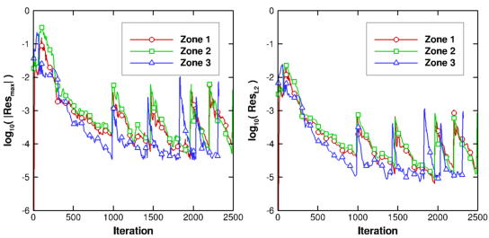
The convergence history for Test Case 4, in terms of the maximum residual and the L2 norm of the residual, should appear similar to that shown below. For this case, the residuals decrease about three orders of magnitude in the first 1000 or so iterations, then oscillate about a relatively constant value for the remainder of the iterations. This behavior is not at all uncommon and is often due to the imposition of boundary conditions or limiters.
As noted above, it's usually more meaningful to use a physical quantity of interest when monitoring convergence. For this test case, one of the physical quantities of interest is the mass flow rate. The time history for these parameters is shown in the figure below, where the computed mass flux is plotted as a function of iteration number at the entrances to all three zones, and at the exit of the duct.
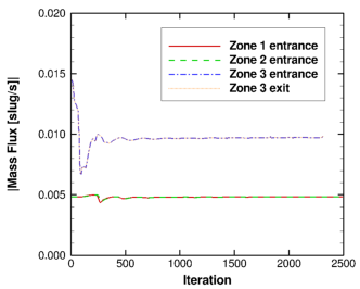
Based on the mass flux results, this case appears to converge within about 750-1000 iterations. Because this is a simple 2-D inviscid flow, with a coarse mesh, it converged quickly in a single run. The various convergence parameters were thus examined only at the end of the run. When running a more realistic configuration, you may need to resubmit your job several times to obtain convergence. To track progress, convergence parameters like those shown in the above figures should be examined at the end of each run. A more complete determination of convergence would also include examination of other physical quantities, such as the pressure distribution along the duct.
Of course, the purpose of the solution process is to determine the features of the flow which can help answer the questions that drove the decision to perform the simulation in the first place. And, as indicated in the previous section, it is important to periodically examine the computed results during a run to help assess convergence and detect numerical problems that might be corrected by adjusting the input.
There are two types of information that can be extracted from the flow simulation - specific quantitative data and qualitative patterns. The first type includes things like pressure distributions, drag, and total flow rate. The second type includes, for example, 2-D slices or full 3-D visualization of pressure contours, streamlines, or isothermal surfaces.
All flowfield results computed by Wind-US, including the mean flow variables, turbulence model variables, and chemistry variables, are written into a Common File called a Common Flow (.cfl) file. [As noted previously, Wind-US also supports the use of CGNS files for the grid and flow solution, using the CGNSBASE keyword.] The CFPOST utility is a post-processing tool for examining the contents of the .cfl file.
With CFPOST a wide variety of variables and integrated values may be computed. Listings of quantitative results may be sent to the screen or to a file. PLOT3D files may be created for other plotting packages and post-processors to use in displaying qualitative results. CFPOST can also be used to create x-y, contour, and vector plots directly, with PostScript output. Commands are available to precisely specify the information of interest, the domain of interest, and the units in which the results are to be presented. More details may be found in the CFPOST User's Guide.
The desired results from this calculation were the mass flow rate and the static pressure distribution. The mass flow rate is available in the List Output (case4.lis) file, as output generated via the LOADS keyword. It was then extracted to a GENPLOT file while monitoring convergence. The result was 9.7 × 10⁻³ slug/sec.
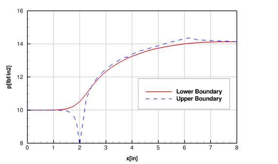
To examine the static pressure distribution, the following CFPOST commands can be used to extract values along the upper and lower walls.
    grid case4.cgd
    solution case4.cfl
    variable x in; p lbf in
   !-----------------------------lower wall
    zone 1
    subset i all j 1 k 1
    zone 3
    subset i all j 1 k 1
    genplot output pdist_lower.gen
    list    output pdist_lower.lis
    list    output pdist_lower.lis.raw raw
   !-----------------------------upper wall
    clear subset
    zone 2
    subset i all j last k 1
    zone 3
    subset i all j last k 1
    genplot output pdist_upper.gen
    list    output pdist_upper.lis
    list    output pdist_upper.lis.raw raw
    quit
All of the output generated by these commands are text files. The user can decide which is the most convenient format to use with external applications. To plot the pressure distribution from the GENPLOT files, issue the following commands within CFPOST.
   @cfpost_setplot.jou
    set plot curve 1 title "Lower Boundary"
    set plot curve 2 title "Upper Boundary"
    plot data pdist_lower.gen merge pdist_upper.gen
When examining results, PLOT3D files are often used as input to other post-processing packages. The following example shows the CFPOST commands used to generate standard PLOT3D grid and solution files as well as a function file containing several variables. The names and units of the function file variables are also written to a file.
    grid case4.cgd
    solution case4.cfl
    units fss
    units inches
    subset i all j all k all
    zone 1 to last
    plot3d xyz pcont.xyz q     pcont.q   2d mgrid unformatted
    variables M;p;T;
    plot3d fun pcont.fun names pcont.nam 2d mgrid unformatted
    quit
The first units command selects the foot-slug-second system
of units, while the second units command resets the length
unit to inches. Thus, the PLOT3D grid file will be in inches and
the pressure will be in units of psi.
Because no variables were selected prior to the first plot3d
command, the solution file will contain the standard PLOT3D
non-dimensional q-variables.
Exactly four (or five) dimensional variables could be selected and
written to a 2d (or 3d) dummy q-file.
The function file format is more flexible in that it allows for an
arbitrary number of variables. Some post-processing programs will
also read the file containing the names of the function file
variables, making it easier to remember what data is stored.
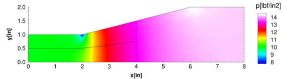
CFPOST can also be used to visualize the solution along prescribed cut planes. This procedure involves the creation of a binary GENPLOT surface file, as shown below.
   @cfpost_setplot.jou
    grid     case4.cgd
    solution case4.cfl
    subset i all j all k all
    zone 1 to last
    units fss
    units inches
    variables p
    cut at z 0.83333336E-01
    genplot surface output pcont.gpc overwrite
    plot color contours data pcont.gpc
The cut plane must intersect the z values in the grid file.
Note, however, that the cut command expects a value in the
default length unit (i.e., feet).
The computed static pressure distribution along the upper and lower walls, and the static pressure field, are shown in the figures below.
The steps in the generalized solution process listed earlier may be expanded and restated specifically for Wind-US as follows:
The various input and output files for the tutorial test case may be downloaded from the following link:
The easiest way to download a file is to click on the file name while holding down the shift key, assuming your browser supports this capability. A dialogue box will appear for you to specify the directory and file name. Alternatively, clicking on the file name without holding down the shift key will display the file contents in your window. (Note that binary files will appear as gobbledy-gook.) The file may then be downloaded using the "Save As ..." menu choice of your browser.
Save the downloaded file to an empty directory and then extract its contents. On a UNIX based operating system, this is done by issuing the following command from a terminal session in that directory:
tar xzvf tutorial_files.tgzThe following files will be extracted:
Note that the files case4.mesh.f90 and case4.dat are the only ones actually required. The rest may be created by following the steps described in the tutorial.
The files case4.xyz, case4.q and case4.fun are Fortran unformatted files in IEEE little-endian format created on a Linux workstation, and may not be portable to some systems. The .cgd and .cfl binary files are in Common File Format, and should be portable to any other platform supporting Common Files.
Last updated 30 Sep 2016