
Wind-US may be used with structured grids for axisymmetric, two-dimensional, or three-dimensional geometric configurations. Two-dimensional grids may be used not only for two-dimensional cases, but also for axisymmetric and area variation (quasi-three-dimensional) cases. Unstructured grids may be used only for three-dimensional configurations.
In three dimensions, each zone's computational mesh is comprised of six boundary faces and an interior grid. For structured grids, the mesh points are identified by three indices, usually labeled (i, j, k). In unstructured grids, each individual grid cell, and cell face, is numbered. Boundary conditions for each boundary face must be specified with GMAN or MADCAP before the grid may be used with Wind-US.
Two-dimensional cases may be run using structured grids only. The grid must be oriented such that the maximum k-index of the grid is one. In other words, a two-dimensional grid is defined by four boundary faces and an interior grid labeled by i- and j-indices. The grid must also reside in a non-zero, z-constant coordinate plane. The actual value used will not affect solution convergence or flowfield features, but it will affect flux-related post-processing calculations such as mass flow. For this reason, a value of 1.0 is recommended. Boundary conditions for the four boundary lines must be specified in GMAN or MADCAP.
With structured grids, the effect of area variation on two-dimensional computational models may be computed by using Wind-US's "quasi-three-dimensional" capability, which is activated simply through changes in the z-coordinate. The value of the z-coordinate is the "width" of the field at each grid point; the complete grid therefore represents the "width" variation of the field as a function of x and y. As with two-dimensional flow, the velocity and derivatives in the third direction are set to zero. The important quantity to model is the ratio of cross-sectional areas between two adjacent axial stations. This means that the z-coordinate may be scaled with no effect on the computed flowfield, but a simple translation of the z-coordinates will change the computed flowfield, because the cross-sectional area ratio will be different. As with two-dimensional calculations, the value of the z-coordinate will affect flux-related post-processing calculations.
Axisymmetric configurations may be modeled with structured grids, by using a two-dimensional grid generated at an arbitrary circumferential location on the geometry - e.g., the top centerline. Note that the grid should be generated on only one "side" of the configuration. Once again, the z-coordinate of the grid should be 1.0. The final step in using Wind-US's axisymmetric mode is the specification of the symmetry axis location and the circumferential sweep angle in the input data file. The circumferential sweep angle is the angle of the "pie shape" swept out by the grid about the symmetry axis. Although the value of the sweep angle will not affect the computed flowfield, it will affect flux-related post-processing calculations.
For axisymmetric cases, the velocity and derivative terms in the
circumferential direction are set to zero. To simulate an
axisymmetric geometry with swirl flow, a three-dimensional
grid must be used. Such a grid would only need to model a
portion (i.e., five degrees) of the geometry in the
circumferential direction. See the discussion of
Mass Flow and Grid Areas
for additional details.
Keywords: AXISYMMETRIC
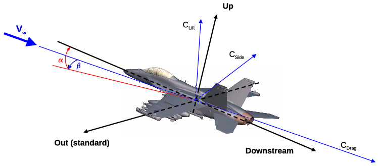
Aerodynamic axes may be specified to ease the set-up and post-processing
of CFD solutions, particularly when starting from a given CAD geometry
and orientation. These axes are defined by the "downstream", "up",
and "out" (or "side") directions as illustrated in the figure below.
The "downstream" direction specifies the vehicle axis and its orientation
from nose to tail. The "up" axis is used to orient the upper surface of
the vehicle. The "out" (or "side") axis is defined by the
"downstream" axis crossed with the "up" axis, however the
"out" (or "side") direction (±) may be specified independently
and will be used when computing the side forces.
The default set of aerodynamic axes is defined as follows: "downstream" (+x), "up" (+y), "out" (+z). To specify the aerodynamic axes with GPRO, select the following options.
  C - Write Output File
  C - COMMON (cgd) File
  D - Modify aeroaxis in existing file
  Enter name of common file (grid.cgd)
  (This will open the grid file and display the current aerodynamic axes settings.)
     Downstream axis is +X
     Up axis         is +Y
     Out axis        is +Z
  Change the current aerodynamic axes? (y/n)
  Enter the downstream direction (+X,+Y,+Z,-X,-Y,-Z)
  Enter the up direction (+X,+Y,+Z,-X,-Y,-Z)
  Enter the side force direction (+X,+Y,+Z,-X,-Y,-Z)
  R - Return to main menu
  S - STOP GPRO
The aerodynamic axes currently set within a grid file can be viewed
using GPRO and are written to the top of the list output file
(.lis) during a simulation.
Flow angles specified in the input data file (.dat) via the
FREESTREAM,
ARBITRARY INFLOW, or
SYNTHETIC JET
keywords are relative to the aerodynamic axes.
The angle of attack (α), defined in the plane formed by the
"downstream" and "up" directions, represents the "vertical" angle
between the freestream velocity and the vehicle axis. Negative, zero,
and positive α values correspond to nose down, level flight, and
nose up conditions respectively. In other words, positive α
yields flow with a +"up" component.
The angle of sideslip (β), defined in the direction
perpendicular to the plane formed by the "downstream" and "up"
directions (ie, "downstream" cross "up"), represents the "lateral"
angle between the freestream velocity and the vehicle axis. Negative,
zero, and positive β values correspond to the wind approaching
from the vehicle left, center, and right respectively. Note that the
± sign of the "out" axis direction has no bearing on the sign
of the sideslip angle, because β is always defined in the
direction formed from the "downstream" axis crossed with the "up" axis.
Flow angles for the
ACTUATOR DISK and
BLEED
keywords are always specified using geometry angles since they are
more closely tied to geometry than wind axes.
Keywords:
FREESTREAM,
ARBITRARY INFLOW,
SYNTHETIC JET
When computing integrated forces and moments via the LOADS keyword:
Forces computed via the
INTEGRATE FORCE
keyword in CFPOST should be equivalent to those from the
LOADS
keyword above, since it reads the aerodynamic axes from the grid
file and implicitly issues the necessary
ORIENTATION
commands.
Keywords:
LOADS
Surface groups are used to reference a surface, or collection of surfaces, which may extend across multiple zones. They offer several convenience factors, including the ability to: refer to named pieces of the geometry (like wing, tail, nozzle, airplane, etc.), use them in the flow solver for requesting LOAD reports, and use them in post-processing with CFPOST and some commercial software. Surface groups can be defined using the CFPART utility. It is usually easier to do this before splitting a grid into multiple zones, simply because there are fewer surfaces to specify. When CFPART is used to split a grid, it will propagate the surface group definitions to the split grid.
Wind-US may be used to solve the Euler equations or the Reynolds-averaged form of the Navier-Stokes equations. [Bush, R. H. (1988) "A Three Dimensional Zonal Navier-Stokes Code for Subsonic Through Hypersonic Propulsion Flowfields," AIAA Paper 88-2830.] All heat transfer and stress tensor terms are retained, and the equations are modeled in full conservation form. The effects of turbulence may be modeled using a variety of algebraic, one-equation, and two-equation turbulence models. Modification of the effective heat transport coefficient due to turbulence is linked to the momentum diffusion coefficient by a turbulent Prandtl number, which is usually assumed to be constant. However, there are a also number of variable turbulent Prandtl number models available.
The fluid may be treated as a thermally and calorically perfect gas, a thermally perfect gas, equilibrium air, or a mixture undergoing a finite rate chemical reaction. For an ideal gas, conventional values are given to the gas constant R and the ratio of specific heats γ, or they may be specified. Effects of gravity (i.e., stratification) and rotation may also be included.
The equation set(s) to be solved must be specified in the input data file.
Keywords:
CHEMISTRY,
GRAVITY,
PRANDTL,
ROTATE,
TURBULENCE
Freestream flowfield conditions - Mach number, pressure, temperature,
angle of attack, and angle of sideslip - must be specified in the
input data file.
The Mach number must be greater than zero, and pressure
and temperature may be specified as static or total values.
These conditions are used to initialize the flowfield at the start of a run.
For external flow problems, they are also applied at all inflow,
outflow, and freestream boundaries during the course of a flow solution.
For this reason, the outermost grid boundary should be far enough away
from the body such that the freestream assumption is valid at the boundary.
Keywords: FREESTREAM
The Reynolds number may be directly specified rather than the
freestream pressure. The input value should be the Reynolds
number based on the freestream velocity U and per unit grid
length. The freestream and reference information is written
to the top of the list output file so that you may confirm that
your input was interpreted correctly.
Keywords: FREESTREAM
Here are a couple of examples.
Case I: Grid is same size as model
Suppose we have the grid for a wind tunnel model, and we want to run it at M∞ = 0.7 and a Reynolds number of 12.1 million (based on the model length). We arbitrarily choose a total temperature of 520 °R (static temperature of 473.6 °R). Knowing the temperature, we can calculate the speed of sound (a = (γRT)1/2) and viscosity (from Sutherland's law). Using the Mach number, we can calculate the freestream velocity. Thus, we have
We now have the Mach number and temperature for the Wind-US input data file, but we still need to calculate the freestream pressure. Using the definition of the Reynolds number (and the ideal gas law),
Note that ReL is the Reynolds number per unit length of the physical model. For our example, if the model length is 10 inches,
We can now calculate P:
We would now like to check our input. If we run Wind-US with the Mach, temperature and pressure specified above, the code will print a Reynolds number and a reference length near the top of the list output file. To obtain the desired Reynolds number, divide Wind-US's value of the Reynolds number by the output reference length and multiply by the model body length. This number may be compared with the desired model Reynolds number.
Case II: Grid is scaled from model size
Let us now assume that we want to run the previous grid at flight conditions, but we want to keep our same old 10-inch grid. We simply need to multiply the pressure by a scale factor. The equation now becomes:
For example, if we want to run a 100-inch wing using our 10-inch grid, S = 10. If we want to run a flight Reynolds number of 26 million, we calculate P as:
One of the options available in Wind-US is the specification of mass flow boundary conditions for subsonic duct analyses. Actual or corrected mass flow may be specified at duct exits, as may back pressure.
Within Wind-US and many post-processors, routines exist which integrate mass flow at desired computational planes. For 3D cases, the desired mass flow may be compared directly with the output from the integration routines.
However, for 2D calculations, the comparison is not so straightforward. There are three cases to consider.
Case I: 2D, Unit Depth
The first case involves running Wind-US on a truly two-dimensional grid of unit depth (z-coordinate is 1.0 everywhere). In this case, the input mass flow should be per unit depth. For example, let's say we want to run a 2D, unit depth model of a duct with a square exit. (If the exit were not square, this model would probably not be very good.) We would like a corrected mass flow of 500 lbm/sec, and our actual model exit depth is 10 inches. If the grid input units are inches, we should ask for a mass flow of 50 lbm/sec. If the grid input units are not inches, simply divide the actual mass flow by the z-coordinate value in inches.
Case II: 2D, Variable Width
When the z-coordinate is the width of the 2D grid, Wind-US adds in the area variation as a source to the 2D equations, making the analysis quasi-three-dimensional. In this case, the actual 3D mass flow should be specified in the input file. The integrated exit area will be (approximately, see the description of mass flow and grid areas) the real duct exit area, if the width has been specified correctly.
Case III: 2D, Axisymmetric
Axisymmetric runs require specification of the symmetry axis location
and the circumferential angle subtended by the 2D grid.
(This angle has no influence on the solution, but it does determine the area
perpendicular to the grid.)
The only reason this angle is an input parameter is so that you will
know what the streamwise area is.
In this case, the real exit geometry is circular, with a corresponding
mass flow.
The ratio of the input mass flow to the actual mass flow
should equal the ratio of the input circumferential angle to 360.
For example, if we are modeling a circular duct with a mass flow of
200 lbm/sec using an axisymmetric model in Wind-US,
and if we specify a circumferential angle of 36 (1/10 of 360),
we should specify a mass flow of 20 lbm/sec
(1/10 of 200 lbm/sec).
Keywords: MASS FLOW,
LOADS
When dealing with subsonic duct analyses, you should be aware that the duct area as represented by the grid may be slightly different from the real area of the geometry being modeled, especially for ducts modeled with quasi-polar structured grids.
The duct area represented by the computational grid is often smaller than the real duct area, which, when running near critical mass flow, may prematurely choke the flow in the CFD solution. If the duct is circular and is modeled with a quasi-polar grid, the area error may be estimated.
Suppose we are modeling a circular duct with a quasi-polar grid using kmax = 33 circumferential points, each of which lie on the perimeter of the real duct at some streamwise station. If the circumferential points are evenly distributed, we may describe this topology as a circle which circumscribes a regular polygon of kmax - 1 = 32 sides. For a circle of radius R circumscribing a regular polygon of n sides, the area of the polygon is
There is no need to worry about this difference for most cases, but you should be aware of its possible effects.
At solid walls, Wind-US uses an adiabatic heat transfer boundary condition by default. A constant wall temperature may also be specified in the input data file.
Through the use of the TTSPEC keyword, point-by-point wall temperature distributions may also be specified on boundary surfaces in structured grids. An auxiliary code, tmptrn, is used to create the wall temperature distribution, and write it into the common flow (.cfl) file.
The thermal conductivity is determined using a constant laminar Prandtl number.
For turbulent flows, constant and variable turbulent Prandtl number
options are available.
The PRANDTL keyword can be used
to specify constant laminar and turbulent Prandtl numbers in all zones.
The VARIABLE TURBULENT PRANDTL
keyword can be used to set constant values or activate variable turbulent
Prandtl number models on a zonal basis.
Keywords:
WALL TEMPERATURE,
TTSPEC,
PRANDTL,
VARIABLE TURBULENT PRANDTL
By default, Wind-US uses Sutherland's law to define laminar viscosity as
a function of temperature.
Keye's formula may be used in addition to Sutherland's law, and
Wilke's law may be used to compute the laminar viscosity for
multi-species flows.
Keywords: VISCOSITY
For turbulent calculations, Reynolds averaging assumptions are used to define a turbulent (eddy) viscosity, which is added to the laminar viscosity in the flow calculations. All the turbulence models available in Wind-US are coupled to the Navier-Stokes equations only through the turbulent viscosity.
Users have a choice of several algebraic, one-equation, and two-equation turbulence models. In addition, various combined RANS/LES models may be used. However, not all turbulence model options are available for both structured and unstructured grids. The Spalart-Allmaras one-equation model and the Menter shear stress transport (SST) two-equation model are the most widely used, tested, and supported models.
Note that a turbulence model (or inviscid or laminar flow) must be specified in the input data file. Wind-US will stop if you do not.
The algebraic turbulence models available in Wind-US for structured
grids are
the Cebeci-Smith model
[Cebeci, T. (1970)
"Calculation of Compressible Turbulent Boundary Layers with Heat and MassTransfer,"
AIAA Paper 70-741]
,
the Baldwin-Lomax model
[Baldwin, B. S. and Lomax, H. (1978)
"Thin Layer Approximation and Algebraic Model for Separated Turbulent Flows,"
AIAA Paper 78-257]
,
and the P. D. Thomas model
[Thomas, P. D. (1979)
"Numerical Method for Predicting Flow Characteristics and Performance
of Nonaxisymmetric Nozzles - Theory,"
NASA CR-3147]
,
which adds a shear layer model to the Baldwin-Lomax model.
After each iteration of the flow solver, these models compute
the turbulent viscosity based on current flowfield quantities.
Note that, because of their dependence on maxima and minima of flowfield
variables, these models produce discontinuous turbulent viscosity
distributions in the computed flowfield and require special numerical
treatment at the juncture of two walls and on computational i-boundaries
(the latter for historical reasons).
Algebraic models should only be used for attached boundary layer flows with
minimal curvature and pressure gradient.
The Baldwin-Lomax model is the most widely used algebraic
turbulence model in Wind-US.
Keywords: TURBULENCE
Because of their efficiency and ability to produce continuous turbulent
viscosity distributions, the one-equation turbulence models in Wind-US
are the models of choice for many engineering applications.
The one-equation models available in Wind-US for structured grids are the
Baldwin-Barth
[Baldwin, B. S. and Barth, T. J. (1990)
"A One-Equation Turbulence Transport Model for High Reynolds Number
Wall-Bounded Flows,"
NASA TM-102847]
and
Spalart-Allmaras
[Spalart, P. R. and Allmaras, S. R. (1992)
"A One-Equation Turbulence Model for Aerodynamic Flows,"
AIAA Paper 92-0439]
models.
The one-equation models available for unstructured grids are that of
Spalart-Allmaras
and the pointwise model of
Goldberg
[Goldberg, U. C. and Ramakrishnan, S. V. (1993)
"A Pointwise Version of the Baldwin-Barth Turbulence Model,"
AIAA Paper 1993-3523;
Goldberg, U. C. (1994)
"A Pointwise One-Equation Turbulence Model for Wall-Bounded
and Free Shear Flows,"
Proc. Int. Sym. Turb., Heat and Mass Trans.,
p.13.2.1, Lisben, Portugal]
.
The Spalart-Allmaras
model is the most widely used one-equation turbulence model, and a practical
choice for many applications.
Keywords: TURBULENCE,
FREE_ANUT
Several two-equation turbulence models are currently available in Wind-US.
The BSL and SST models may be used with both structured and unstructured grids. Most of the k-ε models are only available for structured grids. The realizable k-ε model of Goldberg and the Shih non-linear k-ε model may only be used with unstructured grids.
The Menter baseline (BSL) model is a blend of k-ε and k-ω, with the equations cast in k-ω form. Near viscous boundaries the k-ω model is used, and the k-ε model is used away from walls and in free shear layers. Each equation is solved individually and an iterative method has been used on the implicit side to reduce the factorization error. The Menter shear stress transport (SST) model is similar, but includes a stress limiter term. The SST model is robust, and may be more accurate in mild adverse pressure gradients than some of the other models in Wind-US. Both models may be used with or without compressibility corrections, and freestream values of k and ω may be specified.
For the structured grid k-ε models, several options may be specified to control the initialization procedure, enhance stability, and improve accuracy in adverse pressure gradients and at high Mach numbers.
The Menter shear stress transport (SST) model is considered an industry
standard and is the recommended two-equation model to use.
Keywords: TURBULENCE,
COMPRESSIBLE DISSIPATION,
PRESSURE DILATATION,
FREE_K,
FREE_OM,
K-E keywords
The idea behind combined RANS/LES (Reynolds-averaged Navier-Stokes / large eddy simulation) turbulence models is to improve predictions of complex flows in a real-world engineering environment, by allowing the use of LES methods with grids typical of those used with traditional Reynolds-averaged Navier-Stokes models. The combined model reduces to the standard RANS model in regions of high mean shear (e.g., near viscous walls), where the grid is refined and has a large aspect ratio unsuitable for LES models. As the grid is traversed away from high mean shear regions, it typically becomes coarser and more isotropic, and the combined model smoothly transitions to an LES model.
Several combined RANS/LES models are available in Wind-US.
The combined models may only be used for unsteady flows (i.e., the time
step is a constant).
They are zonal, however, so you can use a combined model in time-accurate
mode in one zone, while using a standard RANS model in steady-state mode
in the other zones.
Keywords: TURBULENCE,
DES,
MDES,
DDES,
LESB,
HYBRID,
PRNS,
DETACHED-PRNS
Through the use of the
TTSPEC keyword,
point-by-point transition data may be specified on viscous walls in
structured grids.
The data represent the percentage of turbulent
viscosity to be added to the laminar viscosity at each grid point.
An auxiliary code,
tmptrn,
may be used to create the transition data, and write it into
the common flow (.cfl) file.
Keywords: TTSPEC
A variety of gas models are available in Wind-US to complete the equation
set.
The fluid may be treated as a thermally and calorically perfect
gas, a thermally perfect gas (frozen chemistry), equilibrium air, or a
mixture undergoing a finite-rate chemical reaction.
Several different chemistry packages are available as files containing
thermodynamic data, reaction rate data, and transport property data.
Keywords: CHEMISTRY
For structured grids, various other models are available in Wind-US to model specific physical features of the geometry.
To simulate fan or compressor discontinuities, Wind-US provides an actuator
disk modeling capability, which acts as a modification to the zone coupling
boundary condition.
The model assumes an infinitesimally thin disk and must be applied at a
coupled zonal interface.
The actual discontinuity is specified in the input data file as a
solid-body rotation or free vortex flow, the effects of which are
applied when transferring flow information between the two specified
zone boundaries.
Keywords: ACTUATOR
Flowfield screens may also be modeled in Wind-US as discontinuities across
coupled zonal interfaces.
In the Wind-US input data file, one must specify the zones and boundaries
between which the screen is located, the solidity of the screen,
and one of several methods for calculating the losses through the screen.
The screen model is not intended for use with choked screens, where the
screen is significantly limiting the mass flow rate.
During the solution start-up phase, it may be necessary to specify a
low solidity, then increase it to the desired value to avoid
strong choking in transients.
Keywords: SCREEN
Heat exchangers may also be modeled at coupled zonal interfaces, using a
procedure similar to that used for actuator disks and screens.
The user specifies the zones and boundaries between which the heat
exchanger is located, the temperature increase across the heat
exchanger, and a static pressure loss coefficient.
Keywords: HEAT-EXCHANGER
Conjugate heat transfer is a term used to describe processes which
involve the thermal interaction between solids and fluids.
Wind-US includes the computational infrastructure needed for
coupling with the
HTX
solid conduction and convection heat transfer
code. A loosely-coupled approach is used whereby the routines pass
heat-transfer and temperature data, which become updated boundary
conditions for the modules.
Keywords: TTSPEC
Two models are available in Wind-US for including the effects of an array of vane-type vortex generators in three-dimensional flow. A vortex generator array consists of one or more vortex generators mounted on viscous wall boundaries.
The Wendt model [Wendt, B. J. (2001) "Initial Circulation and Peak Vorticity Behavior of Vortices Shed from Airfoil Vortex Generators," NASA CR-2001-211144; Dudek, J. C. (2006) "An Empirical Model for Vane-Type Vortex Generators in a Navier-Stokes Code," AIAA Journal, Vol 44, No. 8, pp. 1779-1853] uses a discontinuous change in secondary velocity across a zonal interface boundary in order to simulate the vortices produced by the vortex generators. The model determines the strength of each vortex based on the generator chord length, height and angle of incidence with the incoming flow, as well as the incoming flow core velocity and boundary layer thickness.
The BAY model
[Bender, E. E., Anderson, B. H., and Yagle, P. J. (1999)
"Vortex Generator Modeling for Navier-Stokes Codes,"
FEDSSM99-69 19,
3rd Joint ASME/JSME Fluids Engineering Conference,
San Francisco, California;
Dudek, J. C. (2011)
"Modeling Vortex Generators in a Navier-Stokes Code,"
AIAA Journal, Vol 49, No. 4, pp. 748-759.]
.
is a source term model which models the side force produced by the
vortex generator and adds it to the momentum and energy equations.
This side force automatically adjusts its strength based on the local
flow.
The user specifies the grid points over which the force is to be
applied (i.e., enclosing each vortex generator).
Keywords: VORTEX GENERATOR
The effect of compressor/fan blade rows may be simulated in Wind-US using an actuator duct model, originally developed at MIT. [Gong, Y., "A Computational Model for Rotating Stall and Inlet Distortion in Multistage Compressors," Ph. D. Dissertation, Dept. of Aeronautics and Astronautics, Massachusetts Institute of Technology, Cambridge, Massachusetts, 1999.] Unlike an actuator disk model, in which flow properties change discontinuously across a computational plane, in the actuator duct model the property changes occur within the finite computational region containing the blade rows. The effects of the blades on the flow are modeled by adding body force source terms to the momentum and energy equations.
The user input needed to define the characteristics of the turbomachinery being modeled is read from a set of turbomachinery data files. A separate file is required for each blade row, and currently each blade row must be in a separate zone. The names of the files, and the zone each file corresponds to, are specified using the TURBOSPEC keyword block.
The x-axis of the Cartesian coordinate system used in Wind-US
is assumed to coincide with the axial direction in the cylindrical
coordinate system used in the actuator duct model.
It's also assumed that the i, j, and k
computational indices correspond to the axial, radial, and
circumferential directions, respectively.
And, the zone extent must exactly match the blade; i.e., the leading
and trailing edges of the blade must lie in the upstream and downstream
zonal boundaries.
Keywords: TURBOSPEC
By default, Wind-US initializes the computational flowfield by setting the flow properties at each grid point equal to those specified with the FREESTREAM keyword in the input data file. The same initial conditions are applied at all points in the computational domain, including solid walls, zone boundaries, and freestream boundaries.
Several options in Wind-US lead to non-default initializations, including user-specified inflow conditions, boundary layer initialization, and reinitialization of portions of the flowfield on restart.
Wind-US's ARBITRARY INFLOW keyword was designed to specify flow conditions at arbitrary inflow boundaries. [Recall that the type of boundary, such as arbitrary inflow, is specified using GMAN or MADCAP, and stored in the common grid (.cgd) file, not in the input data file.] However, it may also be used in a variety of ways to specify initial conditions in selected portions of the computational domain that are different from the freestream values. This capability may be useful, for example, when modeling a jet emanating from a solid wall. Zones downstream of the jet exit may have difficulty converging to the proper solution from conditions much different than the jet exit conditions.
To use the ARBITRARY INFLOW keyword as an initialization tool, specify the appropriate parameters and values for a zone as described below, and run Wind-US from scratch (i.e., without an existing flow (.cfl) file). [Note that since the ARBITRARY INFLOW keyword is also used to specify boundary conditions at arbitrary inflow boundaries, a conflict arises if (for some reason) the desired inflow properties are different from those being set as initial conditions. In this case, the ARBITRARY INFLOW keyword can still be used to set initial conditions by setting the number of cycles to be run to zero. Then, after changing the values specified with the ARBITRARY INFLOW keyword to the desired inflow values, simply restart using the initialized flowfield in the newly-created .cfl file.]
There are three ways that the ARBITRARY INFLOW keyword block may be used to modify the default initial conditions.
To provide a better approximation to near-wall flowfields, Wind-US provides a couple of boundary layer initialization options that may help speed the convergence of viscous flows near solid walls.
First, by using multiple IJK_RANGE, XYZ_RANGE, or RTZ_RANGE parameters with the ARBITRARY INFLOW keyword, and setting the range to include not only the inflow boundary but also locations downstream, one can set initial boundary layer profiles all along the viscous walls. Note that using this capability may add many lines to the input data (.dat) file. The INCLUDE keyword may be useful in keeping the main .dat file to a manageable size.
Another option for structured grids is to use the
BL_INIT keyword to specify a
starting location and thickness for a laminar or turbulent boundary layer.
However, this option may only be used on computational j- or
k-boundaries, and only on one boundary in each zone.
Keywords:
ARBITRARY INFLOW,
BL_INIT
Initialization of the solution is a multistep process, much like applying layers of paint to a canvas. It is important to understand the order in which these steps occur so that the desired flowfield can be realized. The initialization proceeds as follows:
In the event that portions of the computed flowfield become "polluted" with unrealistic flowfield data, due to numerical instabilities or other causes, you may wish to reinitialize portions of the flow. Wind-US's reinitialization option enables you to reset the flow conditions in specified zones.
For both structured and unstructured grids, conditions throughout the
zone may be reinitialized to freestream values.
In addition, conditions within specified regions may be reinitialized to
values specified using the ARBITRARY
INFLOW keyword, and/or (for structured grids) the
BL_INIT keyword,
as described above.
Keywords:
REINITIALIZE,
ARBITRARY INFLOW,
BL_INIT
Last updated 30 Sep 2016