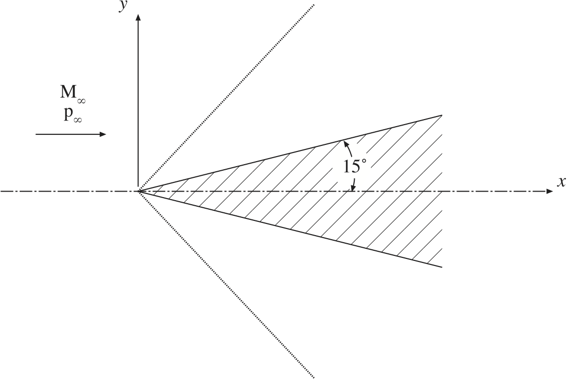
Figure 1. Schematic of supersonic flow over a 15 degree wedge
Figure 1. Schematic of supersonic flow over a 15 degree wedge
Mach 2.0 flow over a 15 degree wedge was used to test the Wind code's ability to compute supersonic inviscid flows and in particular to capture shock waves. Both the structured and unstructured solvers were used and various combinations of spatial operators and flux limiters were tested.
A tar file that contains all the files necessary to run the cases described can be downloaded here, wedge.tar
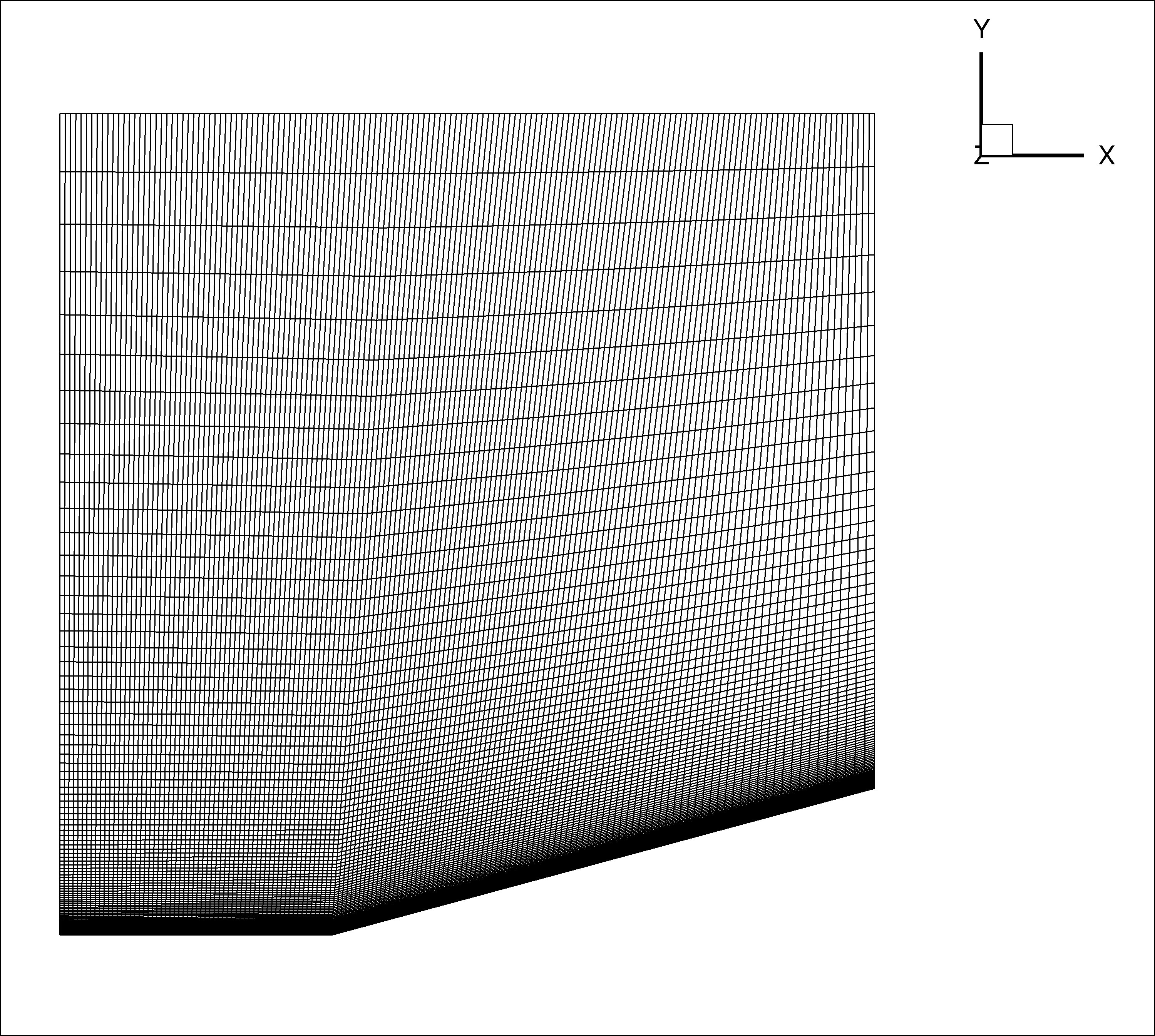
Two grids, a structured grid and an unstructured grid were used. Both grids assume that the flow is symmetric about the centerline of the wedge, and only the upper half of the flowfield is solved. The structured grid was used with both the structured and unstructured solvers to directly compare the solvers on a common grid. Both grids were generated using the Gridgen software package.
The structured grid consists of 153 points in the axial direction, 91 points in the vertical direction and 5 points in the spanwise direction. The grid is relatively uniform in the axial direction and points are clustered near the wedge surface in the vertical direction. No attempt was made to cluster points around the expected shock position, as this is difficult to do in a simple structured grid.
The unstructured grid consists of 5,202 nodes in the 2D plane. The shock position was computed using inviscid theory and grid points were clustered around this line. The resulting plane is extruded one plane in the third direction to create the three-dimensional grid, one cell wide.
 |
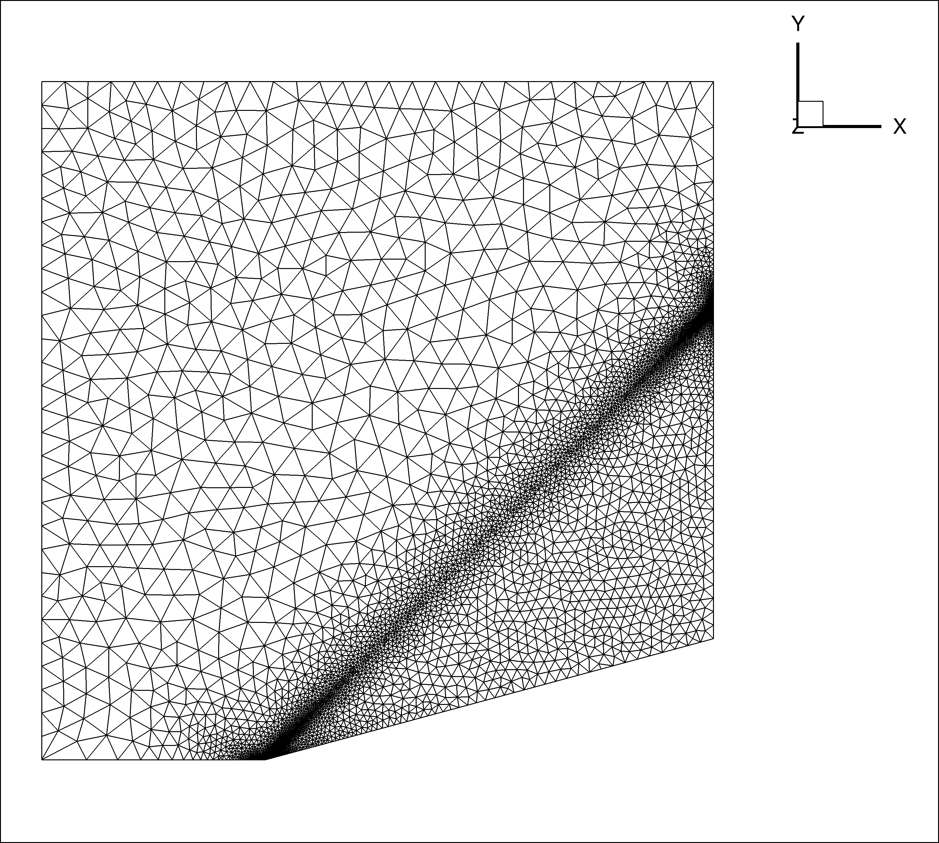 |
| a. Structured grid | b. Unstructured grid |
After the cgd file was exported was created, CFPART was used to generate lines for the Gauss-Seidel implicit solver. The use of the cfpart generated lines in conjunction with the Gauss-Seidel line solver significantly improves convergence. The grid files are listed in table 1 below.
| GridGen (*.gg) | Common Grid (*.cgd) | Preprocessing (*.inp) | |
|---|---|---|---|
| Structured | wedge_st.gg | wedge_st.cgd | wedge_st.inp |
| Unstructured | wedge_un.gg | wedge_un.cgd | wedge_un.inp |
The freestream boundary condition was used for the inflow and upper boundaries. The freestream Mach number was 2.0 and standard atmospheric pressure and temperature were used. At the downstream plane, an outflow boundary with pressure extrapolation was used. The lower boundary used inviscid walls, to simulate both the plane of symmetry on the upstream portion and the inviscid wedge surface on the angled portion.
Eight separate cases were run. Several cases were chosen to provide comparsions between the structured and unstructured solvers. The structured grid can be run used with the unstructured solver and this grid is used for the comparison of solvers. The default settings for the structured and unstructured solvers are different and inputs were selected to compare the defaults for both solvers. In addition cases were selected to show the effect of various TVD limiters available. Table 2, details the input parameters that were varied in the simulations.
| Case 1 | Case 2 | Case 3 | Case 4 | Case 5 | Case 6 | Case 7 | Case 8 | |
|---|---|---|---|---|---|---|---|---|
| Version | 3.139 | 3.139 | 3.139 | 3.139 | 3.139 | 3.139 | 3.139 | 3.139 |
| Solver | structured | structured | unstructured | unstructured | unstructured | unstructured | unstructured | unstructured |
| Grid | structured | structured | structured | structured | structured | unstructured | unstructured | unstructured |
| Time Operator | Default | Default | ugauss line exact_lhs viscous_jacobian full subiterations 6 | ugauss line exact_lhs viscous_jacobian full subiterations 6 | ugauss line exact_lhs viscous_jacobian full subiterations 6 | ugauss line exact_lhs viscous_jacobian full subiterations 6 | ugauss line exact_lhs viscous_jacobian full subiterations 6 | ugauss line exact_lhs viscous_jacobian full subiterations 6 |
| CFL | 0.50 | 0.25 | auto decrease 2 cflmax 500 | auto decrease 2 cflmax 500 | auto decrease 2 cflmax 500 | auto decrease 2 cflmax 500 | auto decrease 2 cflmax 500 | auto decrease 2 cflmax 500 |
| RHS | HLLE second | Roe second | HLLE second | HLLE second | Roe second | HLLE second | HLLE second | Roe second |
| Dissipation | TVD Minmod 2.0 | TVD Minmod 2.0 | TVD Barth 2.0 | TVD Minmod 2.0 | TVD Minmod 2.0 | TVD Barth 2.0 | TVD Minmod 2.0 | TVD Minmod 2.0 |
| Gradients | least_squares | least_squares | least_squares | least_squares | least_squares | least_squares | least_squares | least_squares |
| Boundaries | default | default | implicit boundary on | implicit boundary on | implicit boundary on | implicit boundary on | implicit boundary on | implicit boundary on |
The CFPOST code was used to extract the pressure distribution along the lower, inviscid, surface of the domain. These pressure distributions were plotted against the x-coordinate for comparison between cases. In addtion, contour plots of Mach number are shown.
The input files, grids and resulting solution files for each of the cases are found in table 3.
| Input | Grid | Solution | Post Processing | |
|---|---|---|---|---|
| Case 1 | wedge_case1.dat | wedge_case1.cgd | wedge_case1.cfl | wedge_case1.com |
| Case 2 | wedge_case2.dat | wedge_case2.cgd | wedge_case2.cfl | wedge_case2.com |
| Case 3 | wedge_case3.dat | wedge_case3.cgd | wedge_case3.cfl | wedge_case3.com |
| Case 4 | wedge_case4.dat | wedge_case4.cgd | wedge_case4.cfl | wedge_case4.com |
| Case 5 | wedge_case5.dat | wedge_case5.cgd | wedge_case5.cfl | wedge_case5.com |
| Case 6 | wedge_case6.dat | wedge_case6.cgd | wedge_case6.cfl | wedge_case6.com |
| Case 7 | wedge_case7.dat | wedge_case7.cgd | wedge_case7.cfl | wedge_case7.com |
| Case 8 | wedge_case8.dat | wedge_case8.cgd | wedge_case8.cfl | wedge_case8.com |
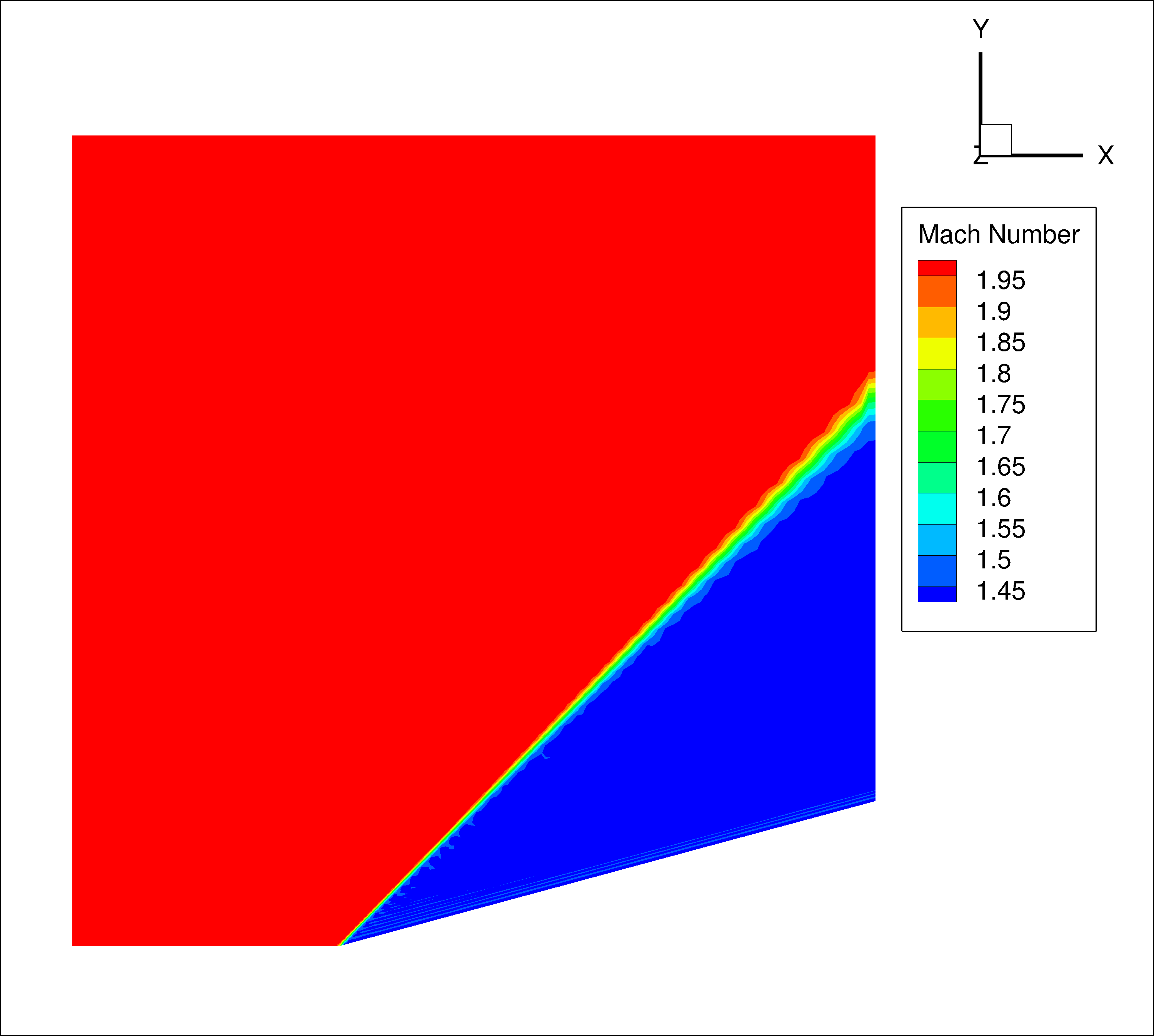
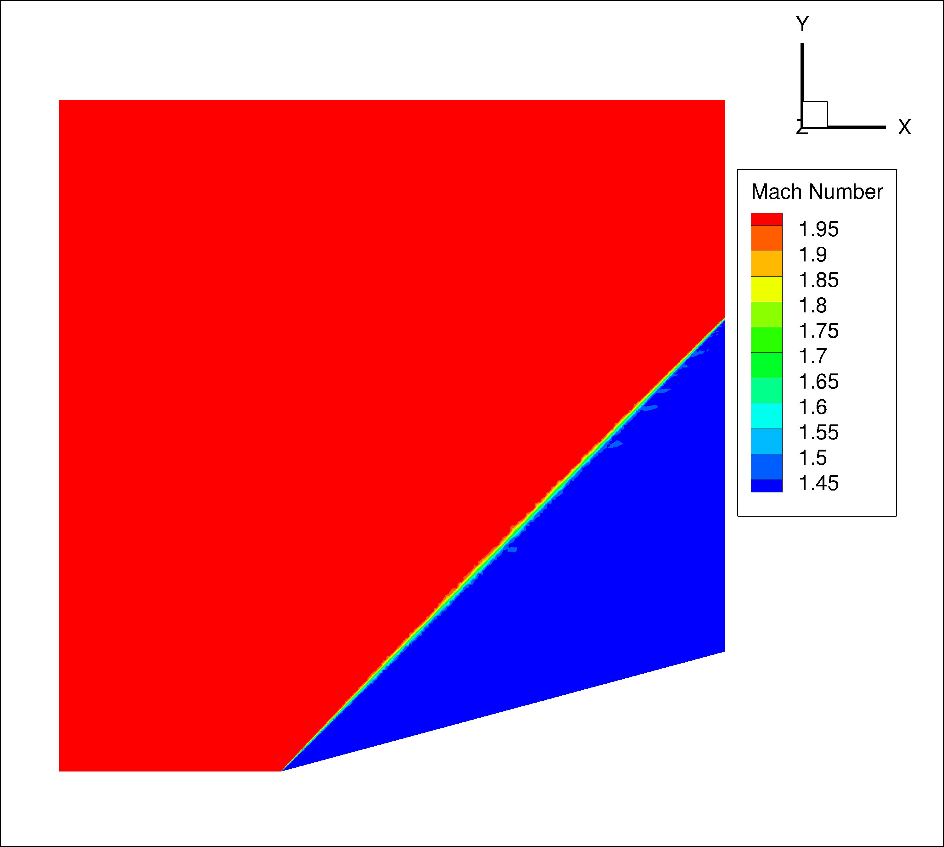
Mach number contours are shown in figure 3. The general characteristic of the flowfield are similar for all three solutions. The Mach 2.0 freestream flow is deflected by the 15 degree wedge causing an oblique shock wave to form. Behind the shock wave, the flow has turned parallel to the wedge surface and the Mach number has been reduced.
The solution obtained by the structured solver on the structured grid is shown in figure 3.a. The shock wave is very thin near the tip of the wedge and grows in thickness as it moves away from the wedge. A similar effect is seen in the solution obtained by the unstructured solver on the structured grid (figure 3.b.). This shock smearing is caused by the increase in the grid cell sizes away from the wedge surface. The solution obtained by the unstructured solver on the unstructured grid shows a very thin shock wave over the entire domain (figure 3.c.). This is because the unstructured grid is clustered near the shock line throughout the domain.
 |
 |
 |
| a. Structured grid, structured solver | b. Structured grid, structured solver | c. Structured grid, structured solver |
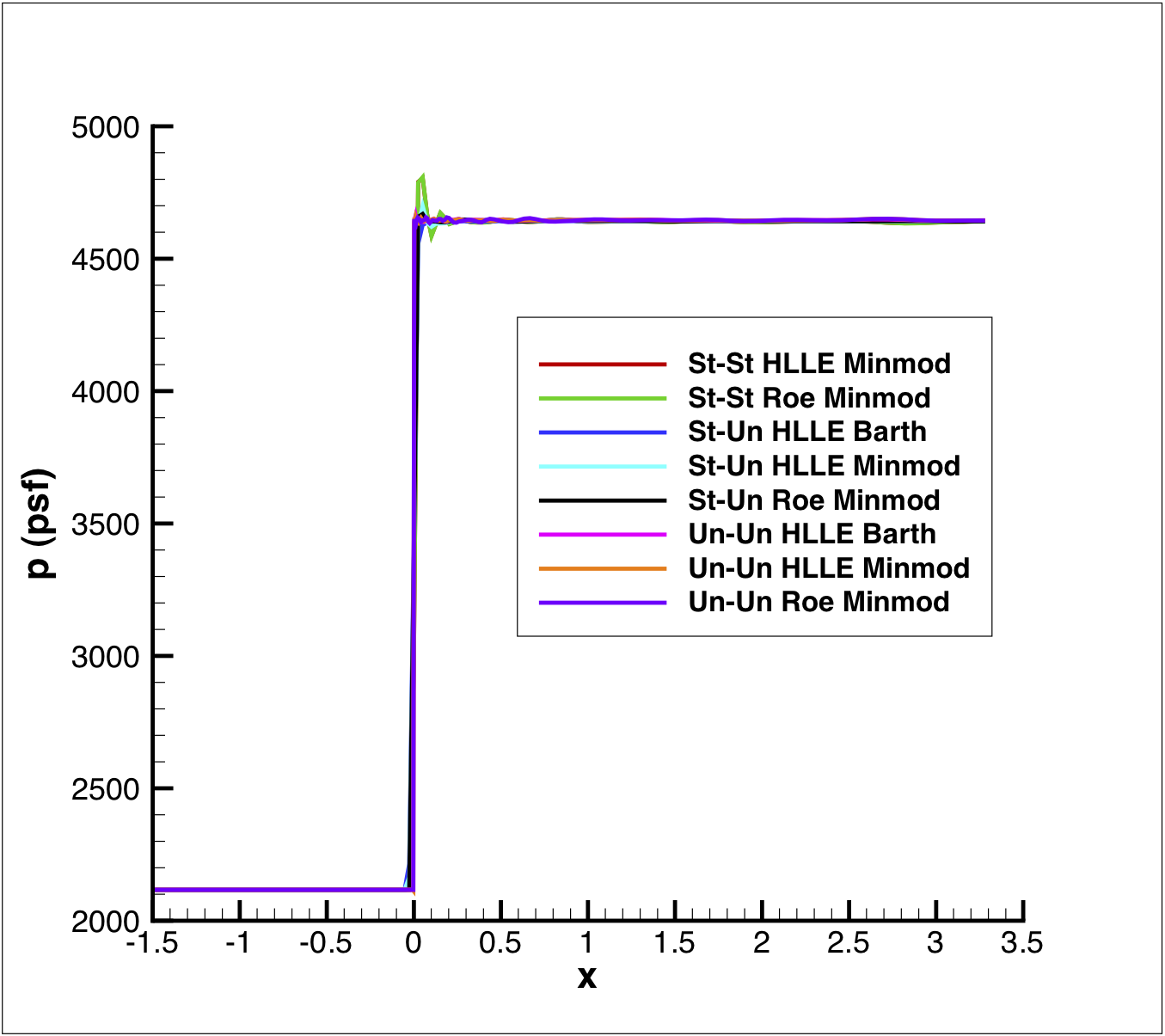
Pressure distributions on the inviscid surface are shown in figure 4. For this simple flow, the pressure should maintain the input freestream pressure until it reaches the leading edge of the wedge surface, x = 0.0, and passes through the shock wave. Behind the shock wave the pressure should immediately jump to the constant post shock pressure. All the cases run exhibit the proper behavior and reach the correct post shock pressure (figure 4.a.).
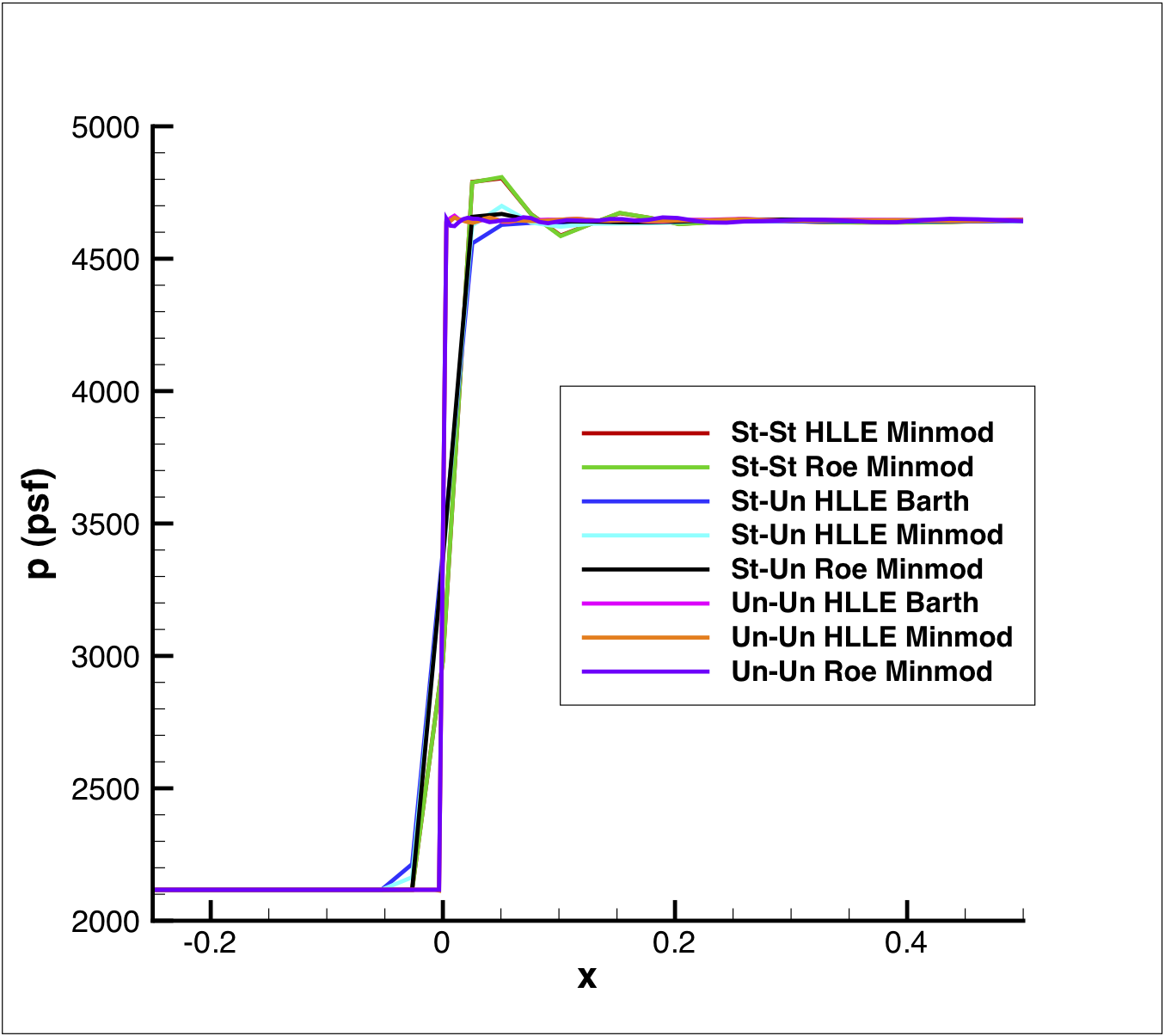
Some small differences between the cases can be seen in the close up region near the shock wave (figure 4.b.). The discontinuous jump in flowfield variables at the shock wave causes problems for almost all numerical schemes. The Wind-US solutions exhibit the classic oscillation in pressure (and other quantities) behind the shock wave. The total variation diminishing (TVD) limiters used in the code minimize these oscillations. For the cases shown here the limiter's compression factor was set to 2. Higher values yielded more oscillation behind the shock and lower values increased the smearing and dissipation around the shock. While the difference are subtle, the Barth limiter, which is only available in the unstructured solver, appears to have the best results.
 |
 |
| a. entire domain | b. close up of shock |
The effect of the grid type and grid distribution can be seen in figure 5. Both the structured and unstructured grid were run using the unstructured solver. Both solutions used the HLLE right-hand side and Barth TVD limiter. The solution using the unstructured grid has a sharper discontinuity, less shock smearing. This effect is due to the fine resolution of the shock region with the unstructured grid and demonstrates the added flexibility inherent in unstructured simulations. It is anticipated that a structured grid tailored to resolve the shock wave would yield a similar solution.
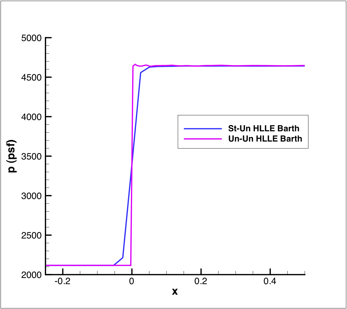
Figure 5. Effect of grid type on the pressure distribution
The accuracy of the structured and unstructured solvers are compared using the structured grid (figure 6.) Both the HLLE and Roe schemes are compared using the minmod TVD limiter. All the solutions are very similar, with the exception of the structured solver's Roe scheme, which produces a stronger post-shock oscillation.
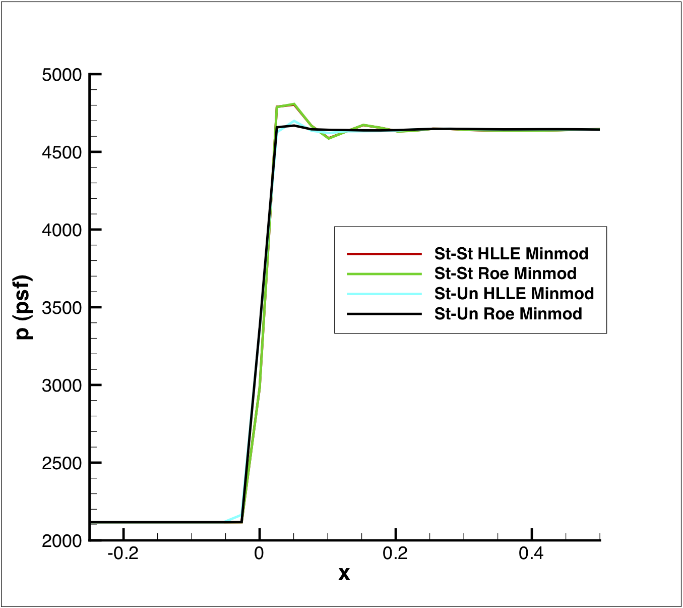
Figure 6. Effect of solver type on the pressure distribution
The accuracy of the Wind-US code was demonstrated for a supersonic inviscid flow containing shocks. Both the structured and unstructured solvers available in Wind-US provided accurate solutions to the problem. Small differences were seen between various numerical scheme and TVD limiter settings. But, the largest factor affecting the accuracy of the solution was the grid resolution of the shock wave. The unstructured solver enables more flexible gridding and easier resolution of the shock wave for this problem.
This validation test case was performed by James R. DeBonis, MS 5-12, NASA Glenn Research Center, 21000 Brook Park Road, Cleveland, Ohio, 44135.