This is the second in a series of validation cases for the new Chien k-epsilon model in WIND. Following the examination of a turbulent flat plate flow case including a grid-sensitivity study, the transonic diffuser problem was chosen as a representative internal-flow case which allows for some experimentation with the compressibility and stability options. As with the flat plate results, the Chien model results were found to be consistent with those from the previous NPARC implementation and compared well with the experimental data.
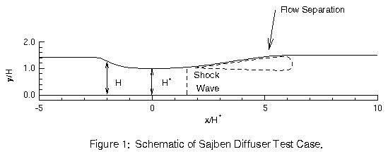
The flow fields being modeled are the weak- and strong-shock diffuser cases of Bogar, Sajben, and Kroutil (1983). Figure 1 is a schematic of the two-dimensional diffuser geometry. This configuration had an entrance to throat area ratio of 1.4, an exit to throat area ratio of 1.5, and a sidewall spacing of approximately four throat heights. Suction slots were placed on the side walls of the constant area sections upstream and downstream of the diffuser to minimize three-dimensional effects. Streamwise slots were also placed along the top corners of the diffuser to maintain a two-dimensional flow. Time-averaged static pressure distributions on the top and bottom diffuser walls were measured using pressure transducers, and separation and reattachment locations were obtained through the use of oil-flow techniques. Velocity profiles were obtained using a laser Doppler velocimeter.
Although this geometry was tested both with and without externally applied oscillations, only the steady-state flow of the unexcited cases was modeled numerically. These flows were characterized by the ratio, R, of exit static to inflow total pressure. For the weak-shock case the value of R was 0.82 and for the strong-shock case it was 0.72. The table below lists the WIND inflow/outflow conditions used for these calculations:
| Inflow | Ouflow | ||
| Total Pressure (psia) | 19.50 | Static Pressure (psia) (weak shock) | 16.05 |
| Total Temperature (R) | 500.00 | Static Pressure (psia) (strong shock) | 14.10 |
| Mach Number | 0.90 |
| Pressures (weak shock) | sajwpres.data |
| Velocity profiles (weak shock) | sajwvel.data |
| Pressures (strong shock) | sajspres.data |
| Velocity profiles (strong shock) | sajsvel.data |
All of the archive files of this validation case are available in a Unix tar file: transdif02.tar. The files can then be accessed by the commands:
tar -xvof transdif02.tar
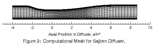
Both cases were computed using the 81 x 51 grid shown in Figure 2. This corresponds to the coarse mesh used in the investigation conducted by Georgiadis, Drummond and Leonard (1994) using the PARC code. They found the grid to be sufficiently clustered in the vertical direction such that the first point off the wall resided inside the laminar sublayer. The grid file uses the Plot3d format (2d, mgrid, unformatted).
| PLOT3D | sajben.x.feet |
| Common Grid | sajben.cgd.feet |
Computations of the weak-shock flow were performed first, then the downstream pressure was increased to obtain the strong-shock solutions. For each case, the following procedure was used: 1) initialize the flow field to uniform conditions, 2) run for 5000 iterations in laminar mode with a low downstream pressure (P=2.50 psia) to establish a supersonic flow, 3) set the proper downstream pressure for the weak-shock case and run for 1000 iterations using the SST turbulence model, 4) initialize the Chien k-epsilon turbulence model from the SST turbulent viscosity and run for 10000 iterations, 5) set the proper downstream pressure for the strong-shock case and run the model for another 10000 iterations starting from the solution obtained in the previous step.
| WIND input data files | sajben.dat |
All calculations were computed using a CFL number of 1.0. Attempts to initialize the k-epsilon model from the Baldwin-Lomax model failed, because the Baldwin-Lomax model solution reverted back to subsonic flow with a very low turbulent viscosity. No stability problems were encountered with the SST model or with the k-epsilon model when initialized from the SST solution.
| Common Solution | List |
| sajw01i10r.cfl | sajw01i10.lis.Z |
| sajw02i10r.cfl | sajw02i10.lis.Z |
| sajw03i10r.cfl | sajw03i10.lis.Z |
| sajw04i10r.cfl | sajw04i10.lis.Z |
| sajwsst10.cfl | sajwsst10.lis.Z |
| Common Solution | List |
| sajs01i10r.cfl | sajs01i10.lis.Z |
| sajs02i10r.cfl | sajs02i10.lis.Z |
| sajs03i10r.cfl | sajs03i10.lis.Z |
| sajs04i10r.cfl | sajs04i10.lis.Z |
| sajsst10.cfl | sajsst10.lis.Z |
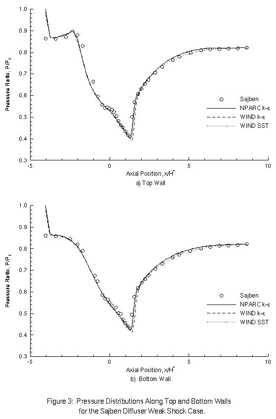
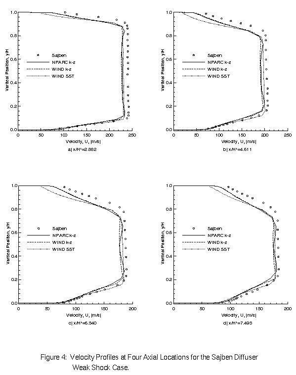
Figure 3 compares the computed pressure distributions along the top and bottom surfaces of the diffuser with the experimentally measured values for the weak-shock case. All of the results compare well with the experimental data. The k-epsilon model predictions of the WIND code match those of the NPARC code, except that the WIND code predicts the shock to occur one or two grid points further downstream. Figure 4 displays the velocity profiles at four axial locations downstream of the shock. From these, it can be seen that both the NPARC and WIND k-epsilon models are in very close agreement. All of the models predict a similar core velocity, but differ in the near-wall region. The results of the SST model better match the velocity data near the lower surface, while the k-epsilon model results more accurately match the data near the upper surface.
Next, the effects of the WIND k-epsilon model correction factors were determined for the strong-shock case. The first of these correction factors is the Sarkar compressibility correction, which provides for an increase in the dissipation rate at higher Mach numbers. The Sarkar correction enables the k-epsilon model to predict an experimentally observed reduction in shear layer growth rate with increasing Mach number. The other correction factor is the variable C_mu option which reduces the turbulent viscosity in regions where the ratio of production to dissipation of turbulent kinetic energy becomes large. This option is derived from algebraic stress modeling and has proven effective near stagnation points, such as the leading edge of an airfoil, where the rapid deceleration of the flow can cause the production term to become very large.
Figure 5 shows that without any correction factors, the WIND k-epsilon model predicts the shock too late and poorly matches the pressure distributions downstream of the shock. Use of the Sarkar compressibility correction improves the prediction of the shock location somewhat, but does little to help the downstream region. The variable C_mu option has the same effect on the shock location as the Sarkar correction, but also improves the downstream pressure predictions. By using the Sarkar correction in conjunction with the variable C_mu option, the shock location is reasonably well matched and the downstream pressure distribution is much improved.
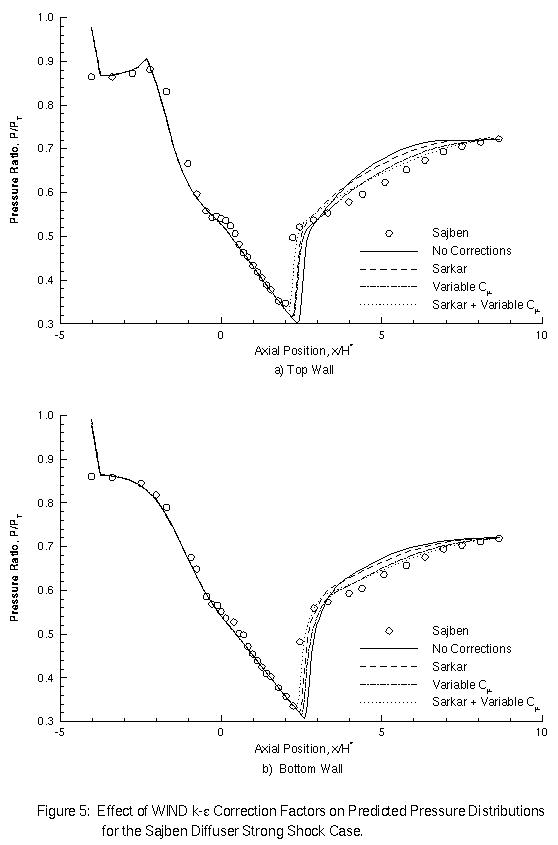
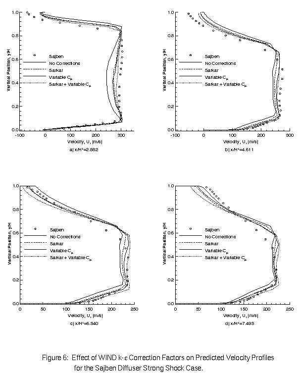
Figure 6 illustrates the effect of the k-epsilon model correction factors on the predicted velocity profiles downstream of the shock. Without any correction factors, the model is unable to match the experimental data near the lower wall and the core flow velocity is underpredicted. Use of either the Sarkar compressibility correction or the variable C_mu option yields improved results both near the walls and in the core. With both correction factors active, some additional improvement is made near the lower wall, while the upper wall region appears to be over-corrected.
Cross-code comparisons of the strong shock results are made in Figures 7 and 8. Two sets of WIND k-epsilon results are plotted. The first set used the same correction factors (Sarkar compressibility correction used, but not the variable C_mu option) as the NPARC code and should be used to compare the new and old k-epsilon implementations. The second series was computed using both correction factors to demonstrate the benefit of using the variable C_mu option. Figure 7 shows that the WIND and NPARC k-epsilon model pressure distributions are again in close agreement, with the WIND code still predicting the shock location one or two grid points further downstream. With the addition of the variable C_mu option, the shock location predicted using WIND agrees well with that using NPARC and the downstream pressure distribution compares better with the experimental data. The WIND SST model also provides improved downstream pressure distributions, but predicts the shock to occur roughly three grid points too far upstream.
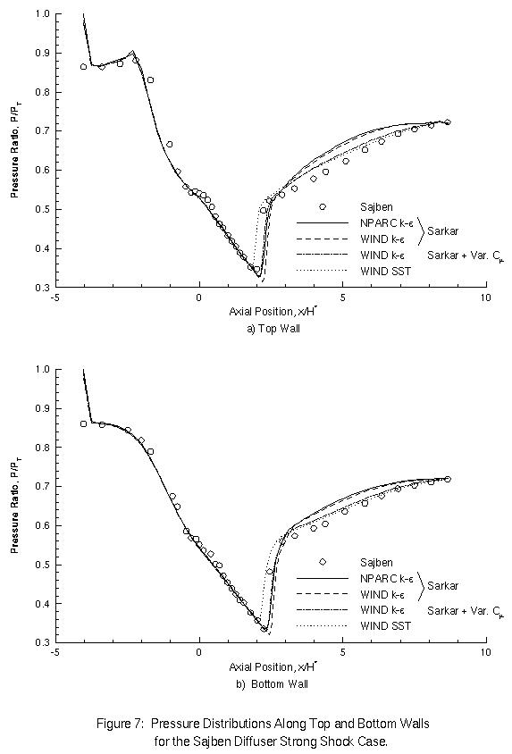
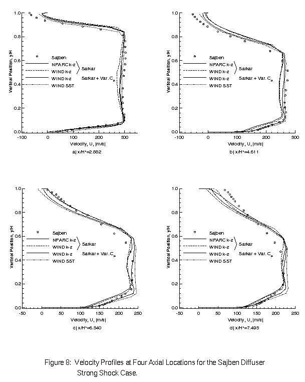
Figure 8 compares the velocity profiles predicted by each model for the strong shock case. The WIND and NPARC k-epsilon results are in close agreement. Use of the variable C_mu option with the WIND k-epsilon model results in better agreement with the bottom wall and core flow data, but sacrifices accuracy near the top wall. The WIND SST model appears to perform the worst further downstream, where it overpredicts the core velocity and is late in its prediction of the flow reattachment.
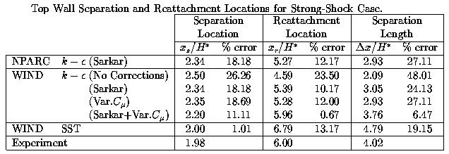
The separation and reattachment locations along the upper surface for the strong-shock case are listed in the following table. These results show that without any correction factors, the k-epsilon model performs quite poorly. Use of either the Sarkar or variable C_mu correction factor reduces the error in the predictions by nearly half. Note that NPARC and WIND k-epsilon results using the Sarkar compressibility correction are comparable. Use of both correction factors improves the k-epsilon results even further. The WIND SST model results show good agreement with the separation location, but the separation length is overpredicted. Of these results, those obtained using the WIND k-epsilon model with both correction factors proved to be the best.
The WIND k-epsilon model validation for transonic diffuser flows has shown that the results obtained with the new implementation are comparable to those obtained using the previous NPARC implementation. Use of the variable C_mu option was found to improve most of the k-epsilon model predictions. Comparison of the NPARC and WIND k-epsilon model results with those from the WIND SST model indicate that the WIND k-epsilon model using both the Sarkar compressibility correction and the variable C_mu option performs the best for the transonic diffuser cases investigated. Though these WIND k-epsilon model results were found to be satisfactory, continued validation of the model is still needed.
Georgiadis, N.J., Drummond, J.E., and Leonard, B.P., "Evaluation of Turbulence Models in the PARC Code for Transonic Diffuser Flows," NASA TM-106391, January 1994.
Bogar, T. J., Sajben, M., and Kroutil, J. C. "Characteristic Frequencies of Transonic Diffuser Flow Oscillations," AIAA Journal, Vol. 21, No. 9, pp. 1232-1240, September 1983.
This validation test case was performed by Dennis Yoder. (216) 433-8716. MS 86-7, NASA Glenn Research Center, 21000 Brook Park Road, Cleveland, Ohio, 44135.