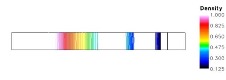
Figure 1. The density contours (normalized by state 4) for the flow in the shock tube
Figure 1. The density contours (normalized by state 4) for
the flow in the shock tube
This validation case is an example case demonstrating the computational process for simulating the unsteady, inviscid flow in a shock tube. It is run in a manner similar to Study # 1, the main difference being that Study # 1 was computed explicitly using Runge-Kutta time stepping, while this study is computed implicitly using the point Jacobi operator.
All of the archive files of this validation case are available in the Unix compressed tar file stube03.tar.gz. The files can then be accessed by the commands:
gunzip stube03.tar.gz
tar -xvof stube03.tar
The grid is a single-block, planar grid generated using the Fortran program stubegr.f. The grid is evenly spaced with a grid density of 100 axial grid points and 7 radial grid points. A Plot3d file (formatted, single-block, whole, two-dimensional) is named stube.x.fmt.
The Plot3d grid file is converted to the common grid file (*.cgd) format using the CFCNVT utility. This is done using the command:
cfcnvt < cfcnvt.x.com
where the file cfcnvt.x.com is a command input file (standard Fortran input unit). A common grid file named stube.cgd is created.
The initial flow conditions are stationary flow with different pressure and density values on either side of the diaphragm. The flow conditions are specified in the WindUS data input file, stube03.dat, described later. The diaphram is located at x = 0.5 ft (grid index I = 50). A 10/1 pressure ratio is specified with the static pressure and temperature values given in Table 1, below.
| Region | Pressure (psia) | Temperature (R) |
|---|---|---|
| 1 | 1.0 | 416.0 |
| 4 | 10.0 | 520.0 |
The INVISCID WALL boundary condition is applied at the J1 and JMAX boundaries of the grid. The FROZEN boundary condition is applied at the I1 and IMAX boundaries of the grid.
The boundary conditions are specified using GMAN. The procedure using the graphics interface is as follows:
Start GMAN.gmanRead in the common grid file by typing at the GMAN prompt.
file stube.cgdSpecify that units are feet / slugs / seconds.
units fssSwitch to graphics mode.
swiDisplay the grid.
Pick SHOW (upper right panel)At this point the grid will be displayed since there is only one grid plane, k=1. Specify the boundary conditions.
Pick SHOW SURFACES
Pick PICK K-PLANE
Pick BOUNDARY COND. (left panel)GMAN defaults to zone 1 since it is the only zone. The sequence is to select the boundary and specify the boundary condition type on that boundary. The initial boundary condition type is UNDEFINED. GMAN also defaults to picking a zone and picking zone 1. It is now waiting for the boundary to be specified.
Pick I1 (lower left panel)At this point, the I1 grid plane is displayed. Since this case is planar, a line is displayed. To select the boundary condition type, execute the following menu choices
Pick MODIFY BNDYAt this point, the bottom panel should contain the text "7 points were changed". The boundary condition specification is now saved for this boundary by the following menu choices
Pick CHANGE ALL
Pick FROZEN
Pick BOUNDARY COND. (top left panel)The common grid file stube.cgd is modified to include this boundary condition specification. The boundary condition specification can be checked by selecting
Pick YES-UPDATE FILE
Pick IDENTIFY PNTS. (left panel)The individual grid points will show up in color to indicate that those points are specified as FROZEN. The boundary conditions for the remaining three boundaries are set in a similar manner. For the IMAX boundary,
Pick FROZEN
Pick BOUNDARY COND. (top left panel)For the J1 boundary,
Pick PICK ZONE/BNDY
Pick PICK IMAX
Pick MODIFY BNDY
Pick CHANGE ALL
Pick FROZEN
Pick BOUNDARY COND.
Pick YES-UPDATE FILE
Pick BOUNDARY COND. (top left panel)For the JMAX boundary,
Pick PICK ZONE/BNDY
Pick PICK J1
Pick MODIFY BNDY
Pick CHANGE ALL
Pick INVISCID WALL
Pick BOUNDARY COND.
Pick YES-UPDATE FILE
Pick BOUNDARY COND. (top left panel)Exit GMAN.
Pick PICK ZONE/BNDY
Pick PICK JMAX
Pick MODIFY BNDY
Pick CHANGE ALL
Pick INVISCID WALL
Pick BOUNDARY COND.
Pick YES-UPDATE FILE
Pick TOP (top left panel)The common grid file stube.cgd is now ready.
Pick END
Pick YES-TERMINATE
As GMAN operates, a journal file gman.jouis created which can later be used as a command file to re-run GMAN. Here this file has been renamed gman.com and GMAN can be re-run as:
gman < gman.com
Creating a command file from scratch represents an alternative to the graphical approach within GMAN.
The computation is performed using the time-marching capabilities of WIND to march in a time-accurate manner to simulate the unsteady flow. A constant time step is specified to be used for each time step. The number of time steps is specified such that the desired time interval is used.
The input data file for WIND is stube03.dat. The keyword inviscid indicates that inviscid flow is assumed. The axisymmetric keyword indicates that the flow domain is assumed to be axisymmetric with a waterline of 0.0 feet and a degree of rotation of 5 degrees. The arbitrary inflow keyword block indicates that the static conditions described in Table 1, above, are to be used, with the higher pressure in the upstream half of the shock tube. The implicit jacobi keyword indicates that the time integration is implicit, and that the point Jacobi implicit operator is to be used. The cycles and iterations keywords indicate that one cycle with 500 time steps is to be run. The timesteps keyword indicates that the actual time step in seconds is specified.
The Wind-US flow solver is run. This computation was performed on an HP xw9400 workstation with dual-core 2599 MHZ AMD Opteron Processor and 896 MB of main memory.
The resulting list file is stube03.lis and contains the output from the computation and lists the residual information for all of the iterations. The flow data file is stube03.cfl and contains the final solution.
Information on the convergence history of the L2 residual can be obtained from the list file stube03.lis using the utility RESPLT,
resplt < resplt.nsl2.com
The file resplt.nsl2.com is a command file containing the inputs for RESPLT to output the file nsl2.gen containing the residual history data.
The program CFPOST can now be used to read in nsl2.gen and plot the convergence history.
cfpost < cfpost.nsl2.comFig. 2 shows a plot of the residual history. The residual reaches an asymptotic value; however, notice that the drop in residual is about half of an order of magnitude. This is because the problem is unsteady and the solution is suppose to change over an iteration, which is now truly a time step. Note that the trends shown in this plot are about the same as the L2 residual history seen in Study # 1, which was computed using explicit time stepping.
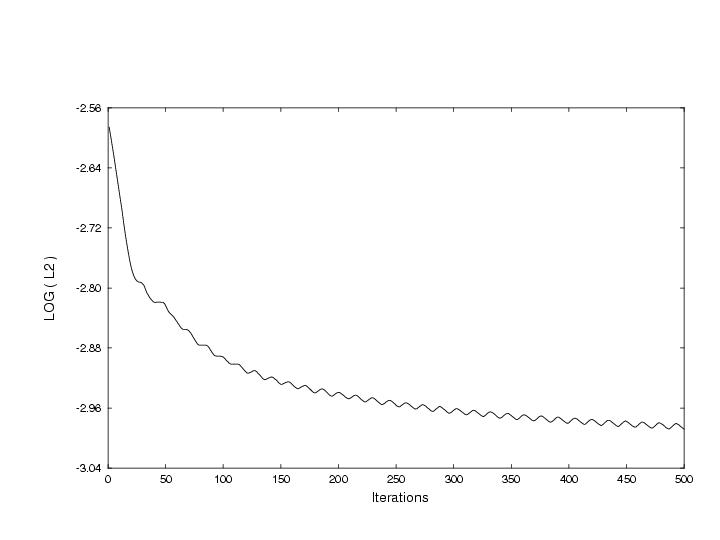
Figure 2. Plot of the L2 residual history.
The CFPOST utility was used to compute and plot the axial distributions of the pressure, density, and Mach number along the shock tube.
The following CFPOST files compute the pressure, density and Mach number, respectively: cfpost.p.com, cfpost.rho.com, and cfpost.mach.com. They also generate corresponding GENPLOT files of the results named p.gen, rho.gen, and mach.gen. So, for example, to create the pressure plot in Figure 3, the following procedure is used. First the pressure is calculated and the p.gen GENPLOT file is written by executing CFPOST:cfpost < cfpost.p.com
Then another CFPOST command file, cfpost.p_comp.com is used to plot these Wind-US results with the theoretical results contained in the GENPLOT file p.theory.gen.
cfpost < cfpost.p_comp.comThe results are shown in Figure 3, below. Similarly, the density along the shock tube is calculated as follows.
cfpost < cfpost.rho.com
Then the CFPOST command file, cfpost.rho_comp.com is used to plot these Wind-US results for density with the theoretical results contained in the GENPLOT file rho.theory.gen.
cfpost < cfpost.rho_comp.com
These results are shown in Figure 4, below. The Mach number in the shock tube is calculated using the same procedure.
cfpost < cfpost.mach.com
Then the CFPOST command file, cfpost.mach_comp.com is used to plot these Wind-US results for mach number with the theoretical results contained in the GENPLOT file mach.theory.gen.
cfpost < cfpost.mach_comp.com
These results are shown in Figure 5, below.
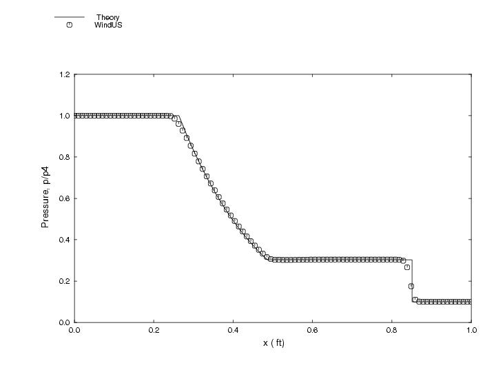
Figure 3. Comparison of the pressure at the final time.
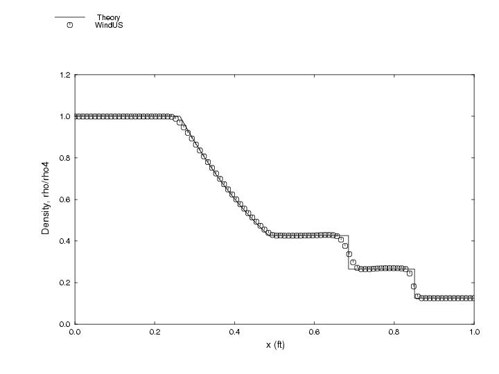
Figure 4. Comparison of the density at the final time.
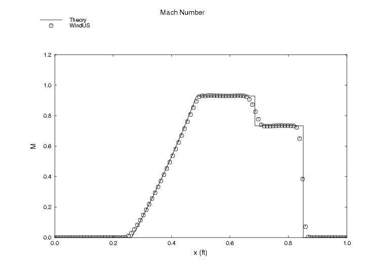
Figure 5. Comparison of the Mach number at the final time.
Julianne C. Dudek
NASA John H. Glenn Research Center, MS 5-12
21000 Brookpark Road
Cleveland, Ohio 44135
Phone: (216) 433-2188
e-mail: Julianne.C.Dudek@nasa.gov