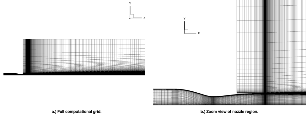
Figure 1. 2-D, structured grid for Seiner nozzle.
In this case, heated flow is passed through convergent-divergent nozzle to produce an ideally expanded, Mach 2.0 jet flow into quiescent air. The nozzle was developed and used by Seiner, et al., for jet noise emission experiments1. It is an axisymmetric, convergent-divergent nozzle with an ideal Mach number of 2.0 and an exit diameter of 3.6 inches. The flow conditions are given in Table 1. The Wind-US simulations used several grids and turbulence models. While there were no experimental data to compare the Wind-US results to, the results are compared to each other.
| Mach | Total Pressure (psia) | Total Temperature (deg R) | Angle-of-Attack (deg) | Angle-of-Sideslip (deg) | |
|---|---|---|---|---|---|
| Jet Inflow | N/A | 115.02 | 563.66 | 0.0 | 0.0 |
| Freestream | 0.01 | 14.7 | 530.0 | 0.0 | 0.0 |
A TAR file containing all the files (grids, solutions, results) for cases presented here is available for download. To unpack the files, use the command:
tar -xzvf Seiner.tz
| Wind-US 3.162 |
|---|
| Seiner.tz |
Since the Seiner nozzle is axisymmetric, a 2-D, structured grid was created to be run in axisymmetric mode; it is pictured in Figure 1. The grid consisted of a nearly 56,800 nodes. The nozzle portion consisted of the 241 points in the axial direction and 81 points in the radial direction. The grid points were clustered radially at the nozzle inner wall (to a nominal grid spacing of y+=1) and the centerline. The grid points were also clustered in the axial direction at the nozzle exit and in regions of curvature along the nozzle wall, including the convergent section.
Figure 1. 2-D, structured grid for Seiner nozzle.
A 3-D version of the structured grid was also created: the grid was extruded in the azimuthal direction 5 degrees and 4 grid cells. This grid is shown in Figure 2. The 3-D structured grid was run using the unstructured solver within Wind-US. Along the centerline, there were only two cells in the azimuthal direction. This strategy addressed the limitation that the Wind-US unstructured solver did not allow the collapsed boundary created along the centerline when the grid was extruded azimuthally. Triangular prisms, extruded in tha axial direction, could have also been used, as they have been shown to work in other axisymmetric cases. The 3-D, Strucutred grid consisted of over 213,000 cells.
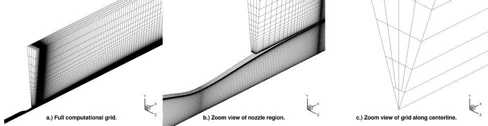
Figure 2. 3-D, structured grid for Seiner nozzle.
Lastly, an unstructured grid was created, consisting of rectangular prisms (along the centerline and nozzle wall surfaces) and triangular prisms, extruded in the azimuthal direction. This grid consisted of just over 489,000 cells. The unstructured grid is shown in Figure 3.
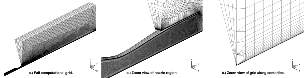
Figure 3. 3-D, unstructured grid for Seiner nozzle.
After creating the unstructured grids, CFPART was used to create lines in the grid to enable the most efficient use of the unstructured line solver. The grid files and CFPART input files are included in Table 4.
| Description | Gridgen File | GMAN Script | CFPART Script | CGD Grid File |
|---|---|---|---|---|
| 2-D, Structured Grid, Structured Solver | Seiner_StrStr.gg | N/A | N/A | Seiner_StrStr.cgd |
| 3-D, Structured Grid, Unstructured Solver | Seiner_StrUns.gg | Seiner_StrUns.gman.com | Seiner_StrUns.cfpart.inp | Seiner_StrUns.cgd |
| 3-D, Unstructured Grid, Unstructured Solver | N/A | N/A | Seiner_UnsUns.cfpart.inp | Seiner_UnsUns.cgd |
The boundary conditions for this nozzle case are shown in Figure 4. The nozzle and freestream inflows were set to their respective total pressure and total temperature listed in Table 1. The 3-D grids used the inviscid wall boundary condition for the sidewalls. Ideally, these boundaries would have used the connect-coupled boundary condition, to allow for flow in the azimuthal direction, but that was not possible for unstrucutre grids using the grid generation tools publically available at this time. The 2-D grid used the inviscid wall boundary condition along the centerline, which is conventional for 2-D, axisymmetric simulations using Wind-US. In the 3-D grids, the centerline was part of the sidewalls (which are inviscid walls) and did not need to be explicitly set. Furthermore, the freestream inflow was set as freestream rather than arbitrary inflow.
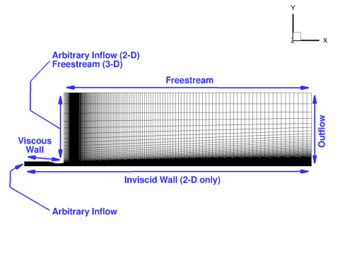
Figure 4. Boundary conditions, shown for the 2-D, structured grid.
Convergence was determined by monitoring the residuals and two flow field quantities key to this case: the velocity and turbulent kinetic energy along the centerline. The algorithm settings used in the DAT file for these unstructured solver cases are listed in Table 5. Note that settings for the structured solver (i.e., choice of RHS method) were different.
| Field | Str-Str SST | Str-Str SST, v2 | Str-Str SST, w/Comp Corr, Press Dilat Off | Str-Str K-epsilon | Str-Str K-epsilon, v2 | Str-Str K-epsilon, w/Comp Corr, Press Dilat Off | Str-Uns SST | Uns-Uns SST |
|---|---|---|---|---|---|---|---|---|
| Version | Wind-US 3.162 | Wind-US 2.22 | Wind-US 3.162 | Wind-US 3.162 | Wind-US 2.22 | Wind-US 3.162 | Wind-US 3.162 | Wind-US 3.162 |
| Grid | 2-D, Structured | 2-D, Structured | 2-D, Structured | 2-D, Structured | 2-D, Structured | 2-D, Structured | 3-D, Structured | 3-D, Unstructured |
| Solver | Structured | Structured | Structured | Structured | Structured | Structured | Unstructured | Unstructured |
| Iterations | 20,000 | 20,000 | 20,000 | 10,000* | 10,000* | 10,000* | 25,000 | 20,000 |
| Convergence Order | 9 | 9 | 9 | 9 | 9 | 9 | 9 | 9 |
| Method | Default | Default | Default | Default | Default | Default | IMPLICIT UGAUSS LINE EXACT_LHS VISCOUS JACOBIAN FULL CONVERGE FREQUENCY 11 SUBITERATIONS 6 | IMPLICIT UGAUSS LINE EXACT_LHS VISCOUS JACOBIAN FULL CONVERGE FREQUENCY 11 SUBITERATIONS 6 |
| CFL | 1.0 | 1.0 | 1.0 | 0.25 | 0.25 | 0.25 | AUTO CFLMIN 2 CFLMAX 10 | AUTO CFLMIN 2 CFLMAX 10 |
| Limiters | Default | Default | Default | DQ LIMITER ON DRMAX 0.2 DTMAX 0.2 | DQ LIMITER ON DRMAX 0.2 DTMAX 0.2 | DQ LIMITER ON DRMAX 0.2 DTMAX 0.2 | DQ LIMITER ON RELAX 0.5 | DQ LIMITER ON RELAX 0.5 |
| Dissipation | Default | Default | Default | Default | Default | Default | TVD BARTH 3.0 | TVD BARTH 3.0 |
| Boundaries | IMPLICIT BOUNDARY ON | IMPLICIT BOUNDARY ON | IMPLICIT BOUNDARY ON | IMPLICIT BOUNDARY ON | IMPLICIT BOUNDARY ON | IMPLICIT BOUNDARY ON | IMPLICIT BOUNDARY ON | IMPLICIT BOUNDARY ON |
| RHS | Default | Default | Default | Default | Default | Default | HLLE SECOND, VISCOUS FULL | HLLE SECOND, VISCOUS FULL |
| Gradient | Default | Default | Default | Default | Default | Default | LEAST_SQUARES | LEAST_SQUARES |
| Turbulence Model | SST | SST | SST | CHIEN K-EPSILON | CHIEN K-EPSILON | CHIEN K-EPSILON | SST | SST |
| Turbulence Options | none | none | COMPRESSIBLE, PRESSURE DILATATION OFF | COMPRESSIBILITY OFF; VARIABLE CMU OFF; TVD ORDER 1; INITIALIZE FROM EXISTING; TURBULENT REFERENCE VELOCITY 2.0; MAXIMUM TURBULENT VISCOSITY 80000 | COMPRESSIBILITY OFF; VARIABLE CMU OFF; TVD ORDER 1; INITIALIZE FROM EXISTING; TURBULENT REFERENCE VELOCITY 2.0; MAXIMUM TURBULENT VISCOSITY 80000 | COMPRESSIBILITY SARKAR; VARIABLE CMU OFF; TVD ORDER 1; INITIALIZE FROM EXISTING; TURBULENT REFERENCE VELOCITY 2.0; MAXIMUM TURBULENT VISCOSITY 80000 | none | none |
| Fixer | OFF | OFF | OFF | OFF | OFF | OFF | AVERAGE | AVERAGE |
| *--The K-epsilon solutions were restarted from converged SST solutions. | ||||||||
The options from Table 5 were incorporated into the DAT input files. The input files for the standard SST turbulence model cases listed above are found in Table 6. The other turbulence model options (i.e., Chien k-epsilon, SST with compressibility correction, etc.) are included, but are commented out. The structured grid, structured solver solutions were sequenced to speed up convergence time and demonstrat grid convergence. The grids were run using every fourth grid point, every second grid point, and every grid point in the axial and radial directions.
| Case | DAT File |
|---|---|
| Str-Str SST | Seiner_StrStr.dat |
| Str-Uns SST | Seiner_StrUns.dat |
| Uns-Uns SST | Seiner_UnsUns.dat |
Two flow quantities were output for each case: axial (u-) velocity and turbulent kinectic energy. Post-processing scripts were created to extract each of these flow quantities. Table 7 includes these CFPOST scripts.
| Case | CFPOST Script | Full Post-Processing Script |
|---|---|---|
| Str-Str SST | Seiner_StrStr.cfpost.com | Seiner_StrStr.pp.csh |
| Str-Uns SST | Seiner_StrUns.cfpost.com | Seiner_StrUns.pp.csh |
| Uns-Uns SST | Seiner_UnsUns.cfpost.com | Seiner_UnsUns.pp.csh |
The solutions from the Wind-US cases listed in Table 5 are presented in Figures 5-14 below. Figures 5-6 show the convergence of the Str-Str SST case: Figure 5 shows the L2 residual convergence of the Str-Str SST case; Figure 6 compares the centerline values of axial (u-) velocity and turbulent kinectic energy (TKE) for each grid sequence.
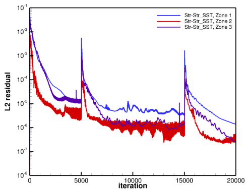
Figure 5. Plot of L2 residuals for determining convergence (Str-Str SST case shown).
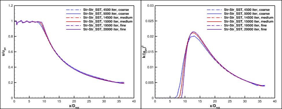
Figure 6. Plot of centerline axial (u-) velocity and turbulent kinetic energy (TKE), showning convergence of Str-Str SST case.
Figures 7-8 show the convergence of the Str-Uns SST case: Figure 7 shows the L2 residual convergence of the Str-Uns SST case; Figure 8 compares the centerline values of axial (u-) velocity and turbulent kinectic energy for each grid sequence. Unfortunately, the Str-Uns SST case did not fully converge, as the peak value of TKE along the centerline continues to increase as the solution is iterated. As will be observed in later figures, the continued increase in centerline TKE is a result of the shear layer unphysically moving towards the nozzle centerline. This problem has yet to be resolved.
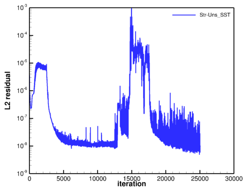
Figure 7. Plot of L2 residuals for determining convergence (Str-Uns SST case shown).
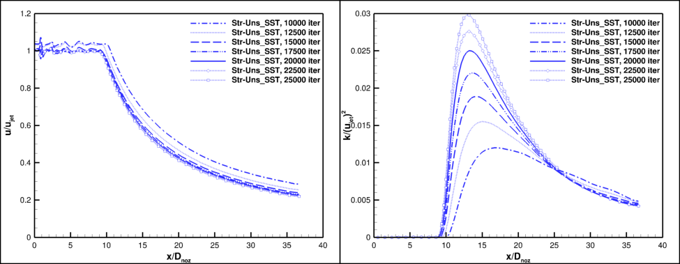
Figure 8. Plot of centerline axial (u-) velocity and turbulent kinetic energy, showning convergence of Str-Uns SST case.
Figures 9-10 show the convergence of the Uns-Uns SST case: Figure 9 shows the L2 residual convergence of the Uns-Uns SST case; Figure 10 compares the centerline values of axial (u-) velocity and turbulent kinectic energy for each grid sequence. Unlike the Str-Uns SST case, the Uns-Uns SST solution did fully converge, as the peak value of TKE along the centerline approaches a constant value as the solution is iterated.
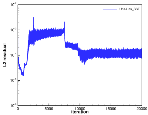
Figure 9. Plot of L2 residuals for determining convergence (Uns-Uns SST case shown).
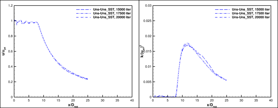
Figure 10. Plot of centerline axial (u-) velocity and turbulent kinetic energy, showning convergence of Uns-Uns SST case.
In addition to running the Seiner jet with Wind-US v3, simulations were performed using Wind-US v2 and GASP2. One improvement of Wind-US v3 over wind-US v2 is that errors in the implementation of the Menter SST turbulence model that affect axisymmetric jet flows were corrected. This is demonstrated in Figure 12: using Wind-US v2 with the SST model, the maximum value of centerline turbulent kinetic energy is on the order of 30% lower than the value predicted by other simulations; using Wind-US v3, the maximum value of centerline turbulent kinetic energy is on par with the other simulations.
Two 2-D, axisymmetric, structured grid simulations of the Seiner jet were performed with GASP using similar methods to what is list for Wind-US in Table 5. The GASP simulations used the SST turbulence model and the K-epsilon turbulence model, neither using compressibility corrections. The GASP solutions are compared to the Wind-US solutions in Figures 11-16.
Experimental data was also available for this case. The experimental centerline u-velocitiy is plotted in Figures 11 and 12. While the Str-Str, non-compressibility correction solutions predict the correct location of the jet potential core breakdown, they all fail to predict the correct velocity slope at the end of the jet potential core, predicting too great a decrease in velocity.
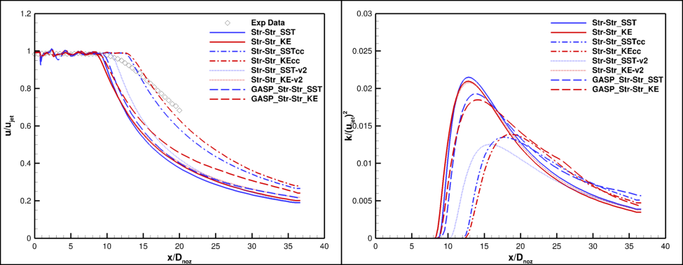
Figure 11. Plot of axial (u-) velocity and turbulent kinetic energy along the centerline, for structured solver solutions.
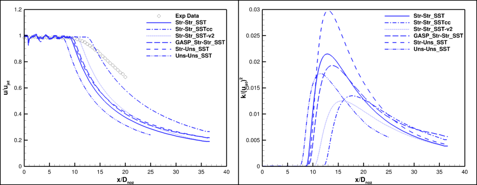
Figure 12. Plot of axial (u-) velocity and turbulent kinetic energy along the centerline, for SST turbulence model solutions.
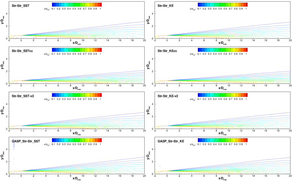
Figure 13. Plot of axial (u-) velocity contours, for structured solver solutions.
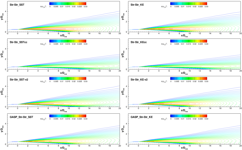
Figure 14. Plot of turbulent kinetic energy contours, for structured solver solutions.
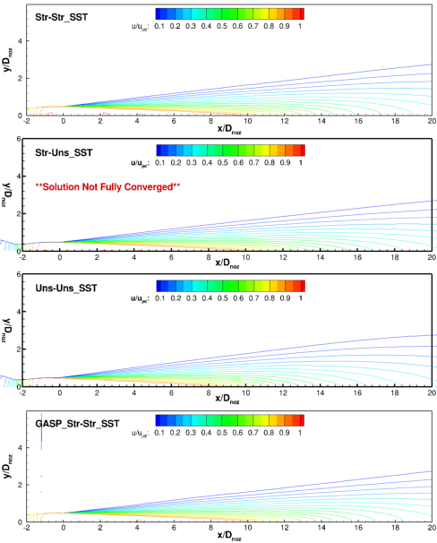
Figure 15. Plot of axial (u-) velocity contours, for SST turbulence model solutions.
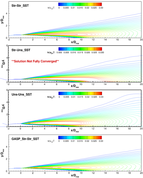
Figure 16. Plot of turbulent kinetic energy contours, for SST turbulence model solutions.
This validation test case was performed by Vance Dippold. Contact: Vance Dippold, MS 5-12, NASA Glenn Research Center, 21000 Brook Park Road, Cleveland, Ohio, 44135.