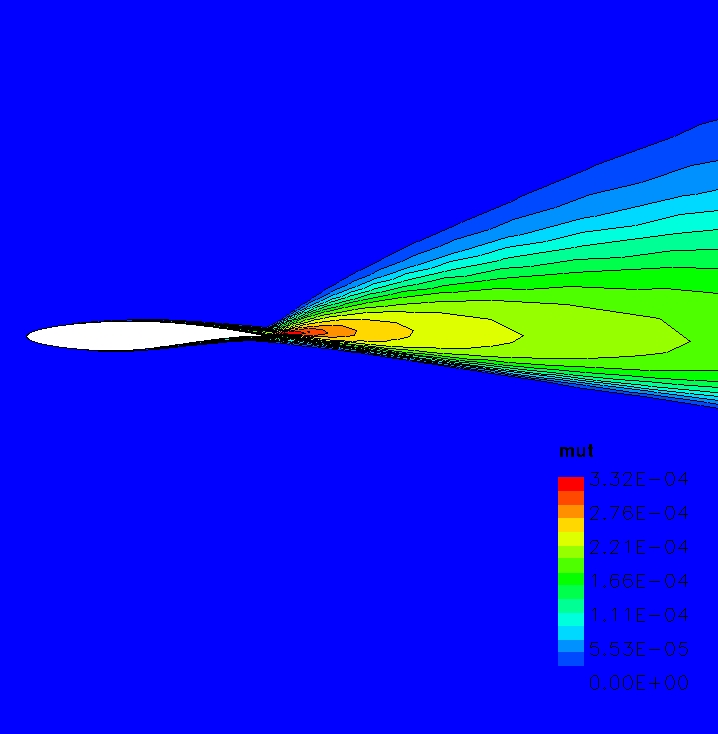
Figure 1. The turbulent viscosity contours for the RAE 2822 transonic airfoil for a simulation computed using the SST turbulence model.
Figure 1. The turbulent viscosity contours for the RAE 2822 transonic airfoil for a simulation computed using the SST turbulence model.
This validation study examines the accuracy of Wind-US for computing two-dimensional, turbulent, transonic flows about an airfoil. Nine different turbulence models are used. The pressure coefficients obtained from the Wind-US solutions are compared with the experimental values obtained by RAE as reported in Ref. 1.
The grid is a single-block, two-dimensional C-grid with dimensions of 369 x 65. It is contained in the file run.cgd and is in the Wind-US common grid file format (.cgd). The airfoil surface and wake are located at the J1 boundary. The I-coordinate starts at the lower downstream boundary, intersects the sharp trailing edge at I33, proceeds along the bottom of the airfoil, around the leading edge, downstream along the top of the airfoil, intersects the trailing edge again at I337, and continues to the outflow boundary. The JMAX grid line is the farfield boundary of the flow domain. The grid is non-dimensionalized by the chord length. Since WIND requires dimensional quantities and assumes English Engineering units, the airfoil grid is assumed to have a chord of 1.0 ft. The grid normal to the airfoil surface is clustered about the airfoil surface to resolve the boundary layer on the airfoil. The first grid point off the wall is at a distance of 1.0E-05 ft from the airfoil surface.
The boundary conditions must now be specified for the grid and this is done with the GMAN utility. First, the boundary condition types are summarized. A VISCOUS WALL boundary condition is applied at the J1 boundary at the airfoil surface, which extends from I33 to I337. The J1 boundary from I1 to I32 is coupled to the J1 boundary from I338 to IMAX (I369) to form the wake region. A FREESTREAM boundary condition is applied at the JMAX boundary, which should all be subsonic inflow at the freestream conditions. The I1 and IMAX boundaries are specified as OUTFLOW boundaries which allows the static pressure to be directly specified and is assumed to be equal to the freestream pressure.
The boundary conditions can be set either by running GMAN in an interactive mode or by creating an input data file and running GMAN in batch mode. Here the input data file gman.com was created and GMAN was executed as:
gman < gman.com
The computation is performed using the time-marching capabilities of WIND to march to a steady-state (time asymptotic) solution. Local time stepping is used at each iteration. The time-marching is performed until iterative convergence is achieved. The convergence criteria was the lift and drag integrated over the airfoil surface.
The input data file is read by WIND at startup to provide WIND with information on performing the simulation. Ten different input data files are available that differ by choice of turbulence models. The input data .dat file names and the corresponding turbulence models used for each case are listed in Table 1, along with some notes on variations on some of the input parameters used. The resulting output .lis files and the solution .cfl files are also given.
| Input File Name | Output File Name | Solution File | Turbulence Model Used | Initial Conditions | Input Notes |
|---|---|---|---|---|---|
| rae.lam.dat | rae.lam.lis | rae.lam.cfl | laminar | freestream | |
| rae.blomax.dat | rae.blomax.lis | rae.blomax.cfl | Baldwin Lomax | freestream | |
| rae.pdt.dat | rae.pdt.lis | rae.pdt.cfl | P. D. Thomas | freestream | |
| rae.bbarth.dat | rae.bbarth.lis | rae.bbarth.cfl | Baldwin Barth | freestream | |
| rae.spalart.dat | rae.spalart.lis | rae.spalart.cfl | Spalart Allmaras | freestream | |
| rae.sst.dat | rae.sst.lis | rae.sst.cfl | Mentor SST | freestream | |
| rae.sst_comp.dat | rae.sst_comp.lis | rae.sst_comp.cfl | Compressible SST | freestream | |
| rae.ke.dat | rae.ke.lis | rae.ke.cfl | Chien k-epsilon | SST solution | CFL = 1.0 |
| rae.rumsey.dat | rae.rumsey.lis | rae.rumsey.cfl | Rumsey-Gatski EASM | Chien k-epsilon solution | CFL = 1.0 |
| rae.cebeci.dat | rae.cebeci.lis | rae.cebeci.cfl | Cebeci Smith | Baldwin-Lomax solution | CFL = 1.0 |
In the above input .dat files, the freestream keyword indicates that the static freestream flow conditions are specified as Mach number, pressure (psia), temperature (R), angle-of-attack (degrees), and angle-of-sideslip (degrees) as listed in Table 2, below. The downstream pressure keyword indicates that the freestream static pressure is to be used at the OUTFLOW boundaries. The turbulence model keyword indicates which urbulence model is to be used. The implicit boundary keyword indicates that implicit boundary conditions are applied on the viscous walls. The dq limiter keyword indicates that changes in the solution over an iteration are limited in order to avoid instabilities due to large transients. The loads keyword indicates that the lift on the airfoil is to be integrated every 10 iterations and displayed in the list file. This will be used to evaluate the convergence of the solution. The converge order keyword indicates that the computation will stop if the L2 norm of the solution drops by 9 orders-of-magnitude. The cycles keyword indicates that 500 cycles will be run. The iterations per cycle keyword indicates that 10 iterations will be run per cycle and residual information will be written to the output list file every 5 iterations. The cfl keyword indicates that a CFL number of 5.0 will be used, unless noted in Table 1. By default, WIND uses local CFL number to determine the time-step size.
This study assumes freestream flow conditions as summarized in Table 1 below. These conditions correspond to a Reynolds number of 6.5 million based on the chord length of 1.0 ft. The static pressure was computed based on the specified Reynolds number and Mach number and an assumed value of static temperature.
| Mach number | Static Pressure (psia) | Temperature(R) | Angle-of-Attack (deg) |
|---|---|---|---|
| 0.729 | 15.80734 | 460.0 | 2.31 |
The computational flow field is initialized with uniform flow corresponding to these freestream conditions.
The WIND solver is run by invoking the wind script. Further details and options for the wind script can be found in the WIND documentation (wind script).
As WIND runs, an output list file is created which contains the output from the computation and lists the residual information for both the flow equations and the turbulence model equations for each iteration. The integrated lift is also output every 10 iterations.
The output list files for runs with each turbulence model are named rae.name.lis, where name corresponds to the turbulence model used, as given in Table 1.
The flow field solution at the final iteration is output to the flow data file. The flow data files for runs with each turbulence model are named rae.name.cfl, as given in Table 1.
Figure 2 shows the comparisons of the pressure coeffiecients on the airfoil for each case compared with experimental results. The pressure coefficient is negative for pressures less than freestream, which occurs on the top of the airfoil. In plots of pressure coefficients for airfoils, the negative of the pressure coefficient is usually plotted to indicate that the lower pressure region is on the top of the airfoil and the high pressure region is on the bottom of the airfoil. More details about post proccessing these solutions can be found in Study 1. Pressure coefficient data from a wind tunnel experiment is available for comparison and is in the GENPLOT file cp.exp.gen.
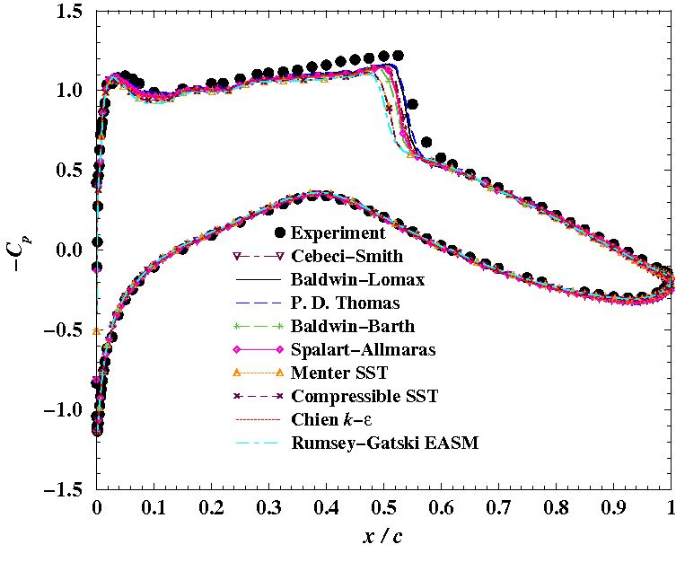
Figure 2. Plot of the pressure coefficients on the airfoil.
The Mach number contours for runs using the Baldwin Lomax, Spalart-Allmaras, SST and Chien k-epsilon turbulence models are shown in Figure 3, below. Again, more details about post processing the solutions can be found in Study 1.
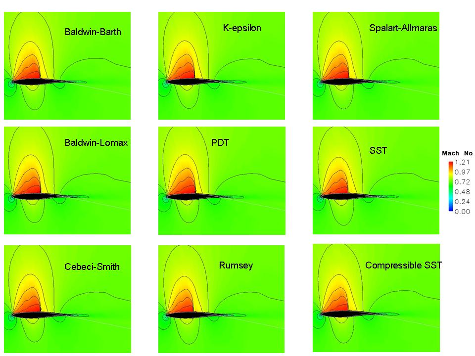
Figure 3. The Mach number contours near the RAE 2822
transonic airfoil.
Most of the smaller files of this validation case (this does not include the grid, output list, and solution files) are available in the compressed tar file raetaf05.tar.gz. The files can then be accessed by the commands:
gunzip raetaf05.tar.gz
tar -xvof raetaf05.tar
1. Cook, P.H., M.A. McDonald, M.C.P. Firmin, "Aerofoil RAE 2822 - Pressure Distributions, and Boundary Layer and Wake Measurements," Experimental Data Base for Computer Program Assessment, AGARD Report AR 138, 1979.
This study was created on February 21, 2008 by Chris Nelson, who may be contacted at:
Voice Mail: 314-373-3311
e-mail: ccnelson@itacllc.com
and Julianne Dudek, who may be contacted at:
NASA John H. Glenn Research Center, MS 5-12
21000 Brookpark Road
Brook Park, Ohio 44135
Phone: (216) 433-2188
e-mail: Julianne.C.Dudek@nasa.gov