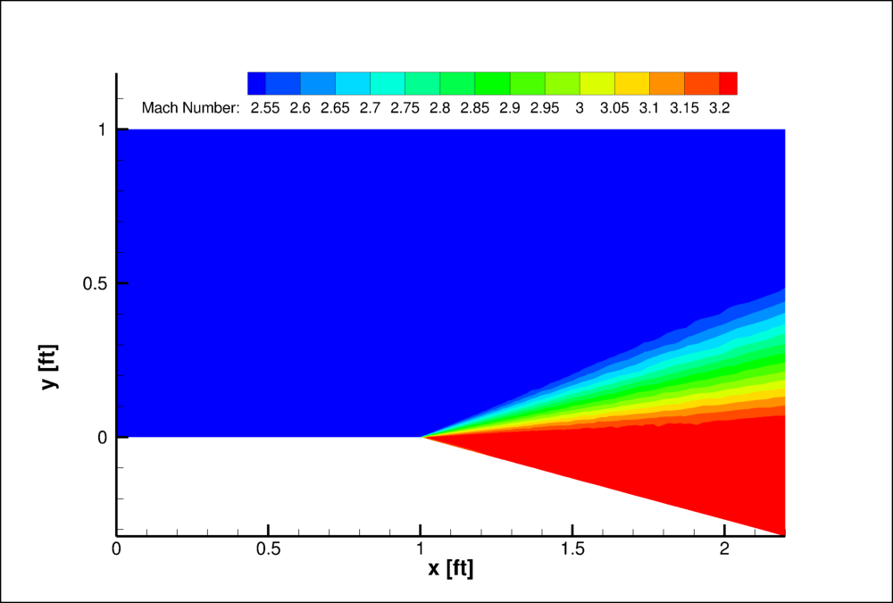
Figure 1. Mach contours of the Mach 2.5 15 Degree Prandtl-Meyer expansion.
Figure 1. Mach contours of the Mach 2.5 15 Degree Prandtl-Meyer expansion.
This is a steady, inviscid expansion case commonly used for validation. This documentation analyzes centerline pressure values at the expansion fan as well as Mach contours.
| Wind-US 3.146 |
|---|
| pm15.tar |
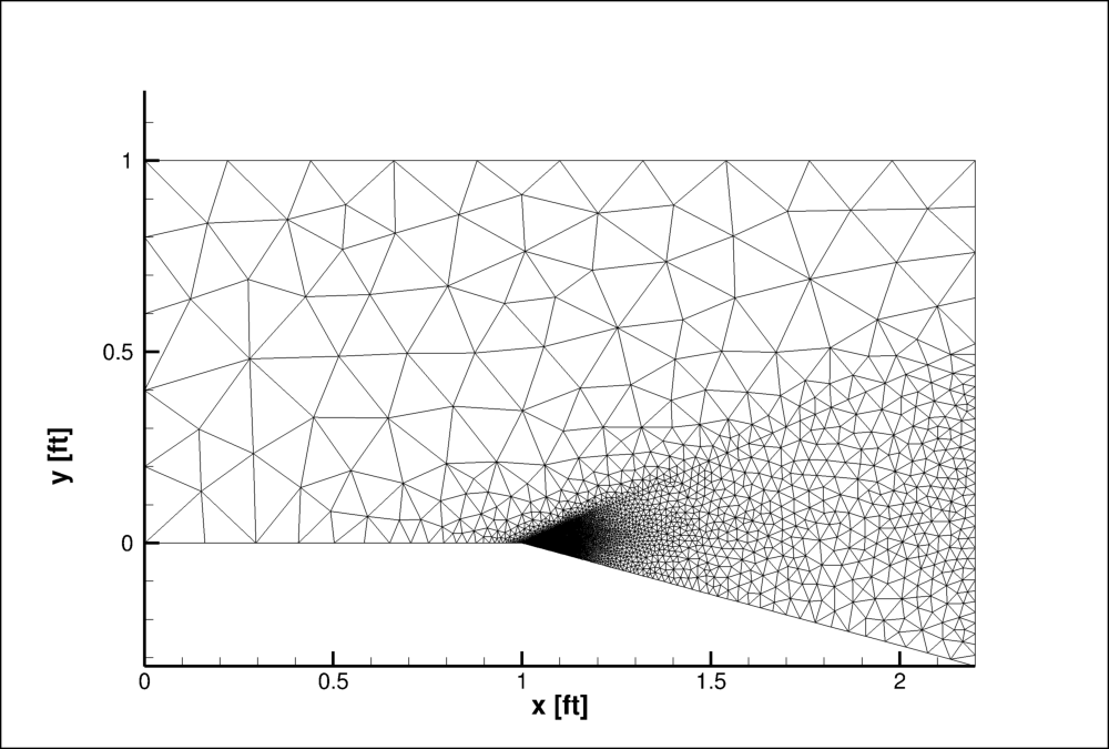
Figure 2. Expansion grid with unstructured (tetrahedral) cells.
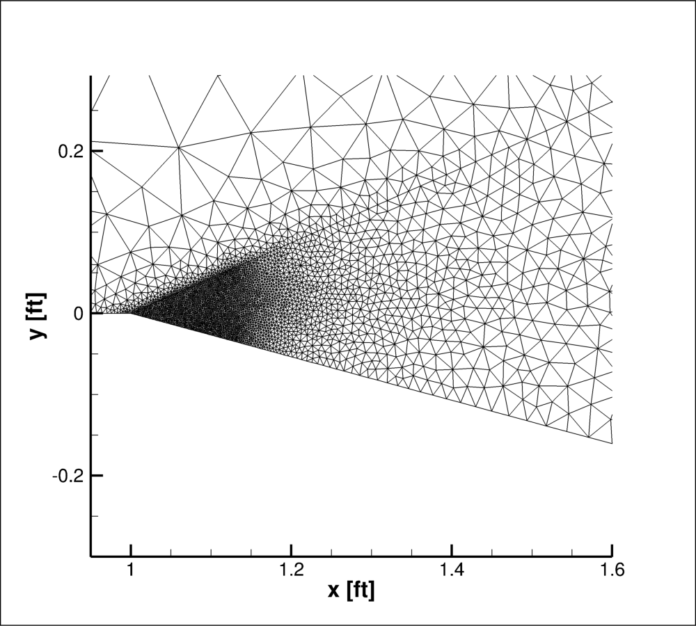
Figure 3. Zoom of the expansion fan.
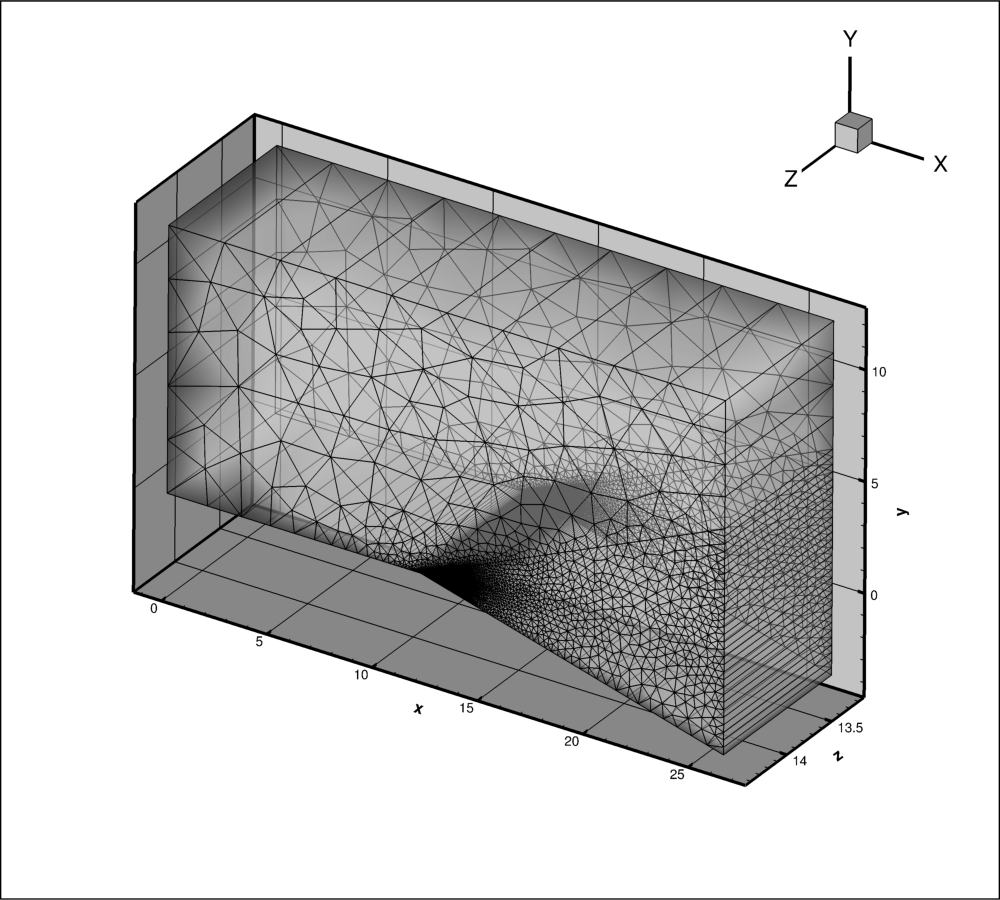
Figure 4. 3D view of the grid.
This grid utilizes dense grid point packing near the expansion fan. The angled shape of the expansion fan makes it favorable to use an unstructured grid. This grid has 7,648 grid points, the majority of are packed near the expansion fan.
Unstructured grids must be extruded into 3D blocks in order to run with Wind-US algorithm. Figure 4 shows a 3D view of this grid.
After the cgd file was exported from Gridgen, CFPART was used to add lines to the grid in preparation to be solved with Wind-US 3.150 code. In Table 1, both the Common and Gridgen versions of the grid are attached as well as the CFPART script.
| Pre-processing | Common Grid | Gridgen | |
|---|---|---|---|
| File | cfpart.inp | pm15.cgd | pm15.gg |
| Pressure (psia) | Temperature (R) | Mach Number | |
| Freestream | 12.0 | 550 | 2.5 |
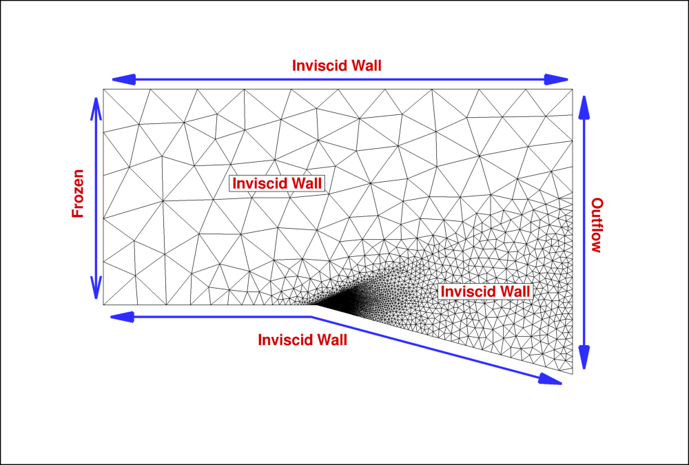
Figure 5. Boundary conditions.
Monitoring the residuals was the main way of determining the convergence of this case. Below are the algorithm settings established in the dat file.
| Field | Parameter |
|---|---|
| Version | Wind-US 3.150 |
| Cycles | 6000 |
| Convergence Order | 8 |
| Method | IMPLICIT UGAUSS EXACT_LHS VISCOUS_JACOBIAN FULL SUBITERATIONS 6 |
| CFL | AUTO CFLSTART 100 CFLMIN 0.1 CFLMAX 1e26 |
| Limiters | DQ LIMITER ON |
| Dissipation | TVD BARTH 3.0 |
| Boundaries | IMPLICIT BOUNDARY ON |
| RHS | HLLE SECOND |
| Gradients | LEAST_SQUARES |
| Turbulence | INVISCID |
| Wind-US 3.150 |
|---|
| pm15.dat |
One post-processing script was used for this case to calculate centerline pressure values at the expansion can. A "results" folder must be created in the scripts' directory in order to create the output files. The cgd and cfl files can be loaded into Tecplot using the Common File Format Loader. Variables can then be measured using the "Probe" tool. "Analyze>Calculate" can be used to calculate more variables and "Data>Alter" can be used to rescale data.
| Script |
|---|
| post_process |
| Computation | Exact | WIND | % Error | Wind-US 3.150 | % Error |
| M2 | 3.2368 | 3.0487 | -5.8125 | 3.2325 | 0.1333 |
| P2/P1 | 0.3274 | 0.3273 | -0.0397 | 0.3275 | -0.0232 |
| Pt2/Pt1 | 1.0000 | 0.7568 | -24.3210 | 0.9938 | 0.6254 |
| rho2/rho1 | 0.4505 | 0.4213 | -6.4883 | 0.4497 | 0.1730 |
| T2/T1 | 0.7269 | 0.7769 | 6.8744 | 0.7282 | -0.1751 |
| Tt2/Tt1 | 1.0000 | 0.9871 | -1.2910 | 1.0000 | 0.0040 |
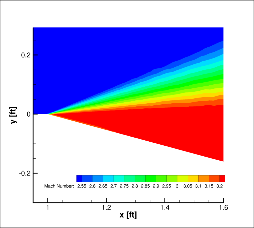
Figure 6. Mach contours zoom of the expansion fan
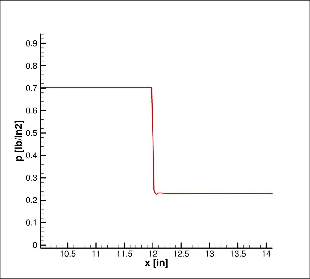
Figure 7. Centerline pressures at the expansion fan
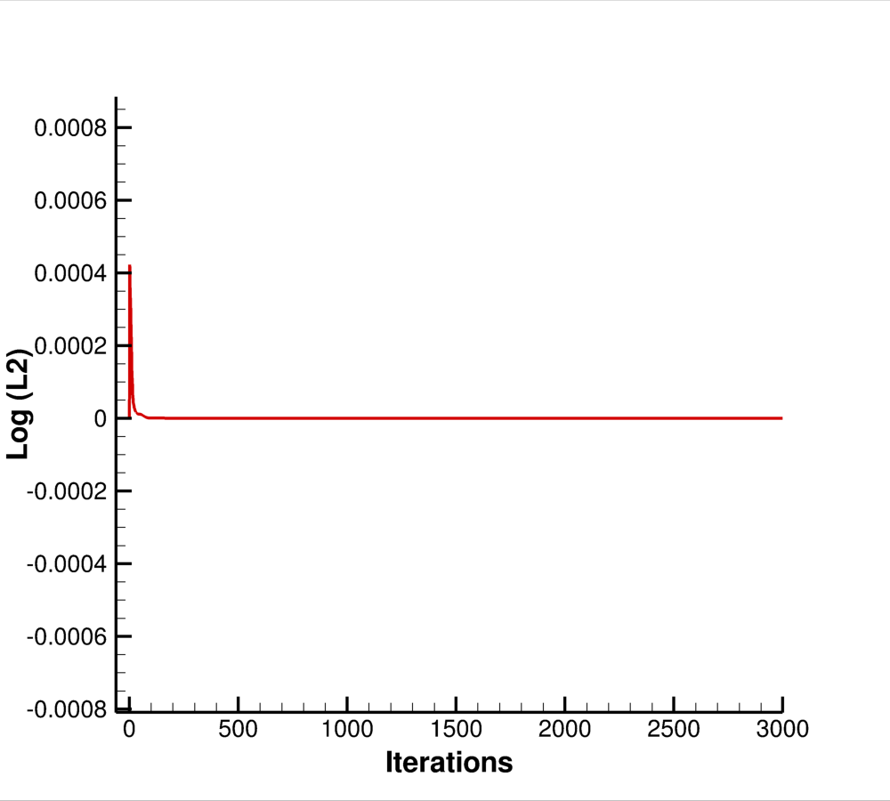
Figure 8. Residual plot for determining convergence
This validation test case was performed by Keven Lenahan. Contact: Manan Vyas, (216) 433-6053. MS 5-12, NASA Glenn Research Center, 21000 Brook Park Road, Cleveland, Ohio, 44135.