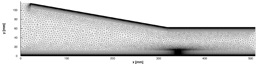
Figure 1: Unstructured grid
The following file is a complete package of grids, solutions, pre- and post-processing scripts, and experimental data used during the course of this validation study. Download the file and extract the folder to see the files.
| Wind-US 4.108 | |
|---|---|
| File | swbli2.tar.gz |
Figure 1: Unstructured grid
This unstructured grid was created with a combination of structured and unstructured mesh elements. The near wall regions were packed with hexahedral layers of cells grown from the wall. Such a wall packing is necessary to resolve the boundary layer and near wall flow features. Therefore it is not recommended that tetrahedra be used to pack important boundary layer regions.
Away from walls, the grid transitions to isotropic tetrahedral cells in the core. High levels of skewness, rapid grid stretching, and abrupt transition from hexahedra to tetrahedra may adversely affect both the convergence characteristics of the solver, as well as the accuracy of a final converged solution. While structured and unstructured mesh elements were applied manually in this grid, most commercially available grid generators allow for an automated transition from near-wall to farfield regions.
This grid was created using Gridgen (swbli.gg) and exported in the Wind-US format (swbli.cgd). The single-zone unstructured grid was partitioned into multiple zones for parallel processing using cfpart tool. The input to the cfpart tool is also provided (cfpart.inp). The tool allows user to create lines which are required for the line Gauss-Seidel implicit solver, which is specified with the implicit keyword. Creating lines is important for viscous problems as it helps the convergence process by increasing the implicit coupling in the line direction and solving the system of equations "simultaneously". For this study, only lines were created and the grid was not partitioned.
| CFPART | Common Grid | Gridgen | |
|---|---|---|---|
| File | cfpart.inp | swbli.cgd | swbli.gg |
| Total Pressure (psia) | Total Temperature (R) | Mach Number | |
| Freestream | 307.48 | 738 | 5.0 |
Figure 2 shows the applied boundary conditions.
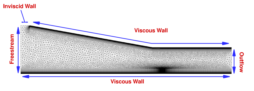
Figure 2: Boundary conditions
The calculations were performed using a first-order scheme for 1000 cycles. At which point, the second-order scheme was turned on and calculations were performed to convergence. Navier-Stokes and turbulence residuals were monitored to determine the convergence.
Table 4 shows a list of input files with appropriate algorithm settings used for the simulations.
| SA | SST |
|---|---|
| SA.dat | SST.dat |
Experimental skin friction and u-velocity data is available for comparison. However, only comparison with skin friction data is presented below due to restrictions on dissemination of the velocity data. The post processing scripts, regardless of the unavailability of the experimental velocity data, extracts calculated velocity data for turbulence model comparisons.
A post-processing bash script, "post_process2", was used to calculate the raw skin friction values for the CFD simulations. Note that a "results" folder must be created in the same directory as the "post_process2" script in order to create the output files. In order to use the bash script, three variables must be set within the script. The first variable, RMode, determines whether the script is being run dynamically as a spawn script during the Wind-US simulation or whether it is being run post-calculation after the Wind-US simulation. The second variable, CMode, sets which variables to be computed. Variables include skin friction coefficient, L2 norm residuals, and select u-velocity profiles. If the u-velocity profiles are computed, use the bash script "zsort" to properly sort the profiles after running "post_process2". Note "zsort" must be located in the "results" folder. The final variable to be set in "post_process2", TMode, sets which turbulence model was run.
In addition to the bash scripts, the cgd and cfl files can be loaded into Tecplot using the Wind-US Common File Format Loader for further analysis. In Tecplot, "Calculate" function in "Analyze" menu can be used to calculate more variables and "Alter" function in "Data" menu can be used to rescale data.
| Skin Friction and Velocity | Sort |
|---|---|
| post_process2 | zsort |
Figure 3 shows Mach number contours for the SA and SST solutions. It can be seen that the SST solution predicts a larger separation compared to the SA solution. Comparing the skin friction coefficient in Fig. 4, it can be seen that the SA solution tends to predict a higher skin friction coefficient compared to the SST solution (with exception of the separation region). However, both Wind-US solutions under predict the skin friction coefficient compared to the experimental data downstream of 360 mm. Residuals were also monitored but not presented here for brevity.
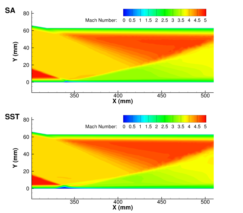 Figure 3: Mach contours comparison |
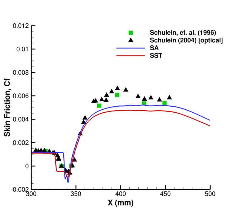 Figure 4: Skin friction comparison |
Schulein, E., Krogmann, P., and Stanewsky, E., "Documentation of Two-Dimensional Impinging Shock/Turbulent Boundary Layer Interaction Flow", DLR Report DLR IB 223-96 A 49, October 1996.
This study was performed by David Friedlander and last updated on January 22, 2015. He may be contacted at:
NASA Glenn Research Center
Inlets and Nozzles Branch
21000 Brookpark Road, M.S. 5-12
Cleveland, Ohio 44135
Phone: (216) 433-3216
e-mail: d.j.friedlander@nasa.gov