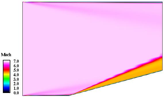
Figure 1. Mach number contours about hypersonic ramp.
Figure 1. Mach number contours about hypersonic ramp.
This study is an example study involving Mach 7.0 flow over a 15 degree ramp and demonstrates the application of several gas models for high-temperature ("real-gas") effects for hypersonic flow applications. Runs A-E use a time-marching algorithm for various air models while run F uses the space-marching algorithm with the equilibrium air model.
All of the smaller archive files (except .cgd, .cfl, and .lis files) of this study are available in the Unix compressed tar file hypramp01.tar.Z. The files can then be accessed by the commands:
uncompress hypramp01.tar.Z
tar -xvof hypramp.tar
The computational process starts from an existing grid. For this study, the grid is a single-block, two-dimensional H-grid with dimensions of 78 x 61. The grid is shown in Fig. 2. below. It is approximatly uniformly spaced in the axial direction and clustered near the walls in the transverse direction. The wall spacing if 1.0E-04 feet. It is contained in a PLOT3D grid file named hypramp.x (unformatted, multi-zone, 3D, whole).
The CFCNVT utility is used to convert the PLOT3D grid file to the common grid file format (.cgd) for WIND. This is done using the command:
cfcnvt < cfcnvt.x.com
where the file cfcnvt.x.com is a command input file. A common grid file named hypramp.cgd is created. For simulating planar flows in WIND, the three-dimensional flow equations are applied. This requires that the grid plane be in the z = 1.0 plane, which is the case in the PLOT3D file hypramp.x.
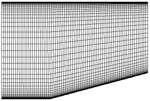
Figure 2. Grid for the hypersonic ramp.
The computational flow field is initialized with uniform flow corresponding to these freestream conditions which are presented in Table 1.
| Mach | Pressure (psia) | Temperature (R) | Angle-of-Attack (deg) | Angle-of-Sideslip (deg) |
|---|---|---|---|---|
| 7.0 | 14.7 | 520.0 | 0.0 | 0.0 |
The boundary conditions must now be specified for the grid and this is done with the GMAN utility. First, the boundary condition types are summarized. A VISCOUS WALL boundary condition is applied at the J1 and JMAX boundaries. The I1 boundary is specified as a FROZEN boundary since the inflow is above Mach 1.0. The IMAX boundary is specified as a CONFINED OUTFLOW boundary to allow for extrapolation of conservative variables since the outflow is primarily supersonic (except in subsonic portion of the boundary laers).
The procedure for setting the boundary conditions using GMAN with the graphics interface is as follows:
1. Start GMAN.
gman
2. Read in the common grid file by typing at the GMAN prompt.
file run.cgd
3. Specify that units are feet.
units fss
4. Switch to graphics mode.
swi
5. Display the grid.
Pick SHOW (upper right panel)
Pick SHOW SURFACES
Pick PICK K-PLANE
At this point the grid will be displayed since there is only one grid plane, K=1. Moving the mouse so that the cross-cursor is near the upper-right most grid point and clicking the left mouse button will cause the coordinates of that point to be displayed in the middle right panel. It should indicate that the coordinates of point (78,61,1) are x = 1.0 ft, y = 1.0 ft, and z = 1.0 ft. Note that the units are feet, which was desired from the units fss command. Also note that z = 1.0 ft, which is required by WIND for two-dimensional flow computations.
6. Specify the boundary conditions.
Pick BOUNDARY COND. (left panel)
GMAN defaults to zone 1 since it is the only zone. The sequence is to select the boundary and specify the boundary condition type on that boundary. The initial boundary condition type is UNDEFINED. Since there is only one zone, GMAN defaults to picking zone 1. It is now waiting for the boundary to be specified.
Pick I1 (lower left panel)
At this point, the I1 grid plane is displayed. Since this case is planar, a line is displayed. To select the boundary condition type, execute the following menu choices:
Pick MODIFY BNDY
Pick CHANGE ALL
Pick FROZEN
At this point, the bottom panel should contain the text "61 points were changed". The boundary condition specification is now saved for this boundary by the following menu choices
Pick BOUNDARY COND. (top left panel)
Pick YES-UPDATE FILE (middle left panel)
The common grid file run.cgd is modified to include this boundary condition specification.
The boundary condition specification can be checked by selecting:
Pick IDENTIFY PNTS. (left panel)
Pick FROZEN
The individual grid points will show up in color to indicate that those points are specified as FROZEN.
The boundary conditions for the rest of the boundaries are set in a similar manner. For the IMAX boundary,
Pick BOUNDARY COND. (top left panel)
Pick PICK ZONE/BNDY
Pick IMAX
Pick MODIFY BNDY
Pick CHANGE ALL
Pick OUTFLOW
Pick BOUNDARY COND.
Pick YES-UPDATE FILE
For the J1 boundary,
Pick BOUNDARY COND. (top left panel)
Pick PICK ZONE/BNDY
Pick J1
Pick MODIFY BNDY
Pick CHANGE ALL
Pick VISCOUS WALL
Pick BOUNDARY COND.
Pick YES-UPDATE FILE
For the JMAX boundary,
Pick BOUNDARY COND. (top left panel)
Pick PICK ZONE/BNDY
Pick JMAX
Pick MODIFY BNDY
Pick CHANGE ALL
Pick VISCOUS WALL
Pick BOUNDARY COND.
Pick YES-UPDATE FILE
While computationally there exists K1 and KMAX boundaries, which are both K1, they do not need to be specified for planar problems.
7. Exit GMAN.
Pick TOP (top left panel)
Pick END
Pick YES-TERMINATE
The common grid file hypramp.cgd is now ready.
As GMAN operates, a journal file gman.jou is created which can later be used as a command file to re-run GMAN. Here this file has been renamed gman.com and GMAN can be re-run as:
gman < gman.com
Creating a command file from scratch represents an alternative to the graphical approach within GMAN. Further, it can be easily modified when the grid changes, such as for grid refinement studies.
The computations for runs A through E are performed using the time-marching capabilities of WIND to march to a steady-state (time asymptotic) solution. Local time stepping is used at each iteration. The time-marching is performed for 8000 iterations. Run F uses the space-marching capabilities of WIND to solve the parabolized Navier-Stokes equations, which require significantly less computational time. The space-marching approach can be used for this case because the flow is predominantly supersonic in the streamwise direction and there is no flow separation in the boundary layer.
The input data files for the WIND runs are presented in Table 2 below. The freestream keyword indicates that the static freestream flow conditions are specified as Mach number, pressure (psia), temperature (R), angle-of-attack (degrees), and angle-of-sideslip (degrees) according to the conditions of Table 1. The turbulence keyword indicates that the laminar viscous flow is assumed. The downstream pressure keyword indicates that the OUTFLOW boundary conditions at the outflow are extrapolated from within the flow domain. The dq limiter keyword indicates that the solution over an iteration will be limited to avoid large changes in the solution. The rhs keyword indicates that the second-order Roe flux-difference splitting is to be used for the explicit flux terms. The tvd keyword indicates that a factor of 1 is to be applied. The cfl keyword indicates that a constant CFL number of 0.5 will be used. By default, WIND uses CFL number to determine the maximum local time-step size. The cycles keyword indicates that 80 cycles will be run. The iterations per cycle keyword indicates that 100 iterations will be run per cycle with residuals printed every 10 iterations. The converge order keyword indicates that the computation will stop if the L2 norm of the solution drops by 9 orders-of-magnitude. The test 128 keyword indicates that the total L2 residual will be monitored rather than the maximum.
The chemistry keyword indicates the gas / chemistry model that is used. By default, WIND uses a calorically perfect air model.
For run F, the cycle and iterations keywords indicate that a cycle cooresponds to one marching surface and a maximum of 200 iterations per cycle (marching surface). The marching keyword indicates that the space-marching algorithm is to be used. The limiter limits the solution at the new plane to be within 86% of the solution on the previous surface. The checkpoint keyword indicates that the solution is to be written to the solution file every 5 marching surfaces. The copy keyword indicates that the initial flow field on a surface is copied from the previous surface. The space marching option automatically changes the rhs to use the physical first method in the marching direction.
| Run | Gas Model | Input Data File |
|---|---|---|
| A | Calorically Perfect Air | run.A.dat |
| B | Thermally Perfect Air. 2-Species Model. | run.B.dat |
| C | Equilibrium Air | run.C.dat |
| D | Frozen Chemistry. 5-Species Model. | run.D.dat |
| E | Finite-Rate Air Non-Equilibrium Chemistry. 5-Species Model. | run.E.dat |
| F | Equilibrium Air. Space-Marching | run.F.dat |
The WIND flow solver is run using the wind script,
wind -runinplace -dat run.A
The steady-state flow was computed for each run. Table 2 lists the names of the input data files for each run. The runs mostly used the default input values for WIND. A CFL number of 0.5 was used for all runs. The computations were performed for 8000 iterations, which generally resulted in the "leveling out" of the convergence histories.
| Run | List File | CFL File | RESPLT File | CPU (sec) |
|---|---|---|---|---|
| A | run.A.lis | run.A.cfl | nsl2.A.d | 906.21 |
| B | run.B.lis | run.B.cfl | nsl2.B.d | 2011.25 |
| C | run.C.lis | run.C.cfl | nsl2.C.d | 1127.25 |
| D | run.D.lis | run.D.cfl | nsl2.D.d | 5069.79 |
| E | run.E.lis | run.E.cfl | nsl2.E.d | 5086.85 |
| F | run.F.lis | run.F.cfl | nsl2.F.d | 33.11 |
The convergence of the solution is examined by monitoring the iteration history of the L2 norm of the total residual of the flow equations. The RESPLT utility is used to read the residual information from the list file,
resplt < resplt.nsl2.com
The file resplt.nsl2.com is a command file containing the inputs for RESPLT to output the GENPLOT formatted plot data file named nsl2.gen of the residuals as a function of the iterations. The x-y plot files for the residual convergence are listed in Table 3. Figure 3 shows the plots of the residuals for runs A through E. All seem to level out with some high-frequency oscillations.
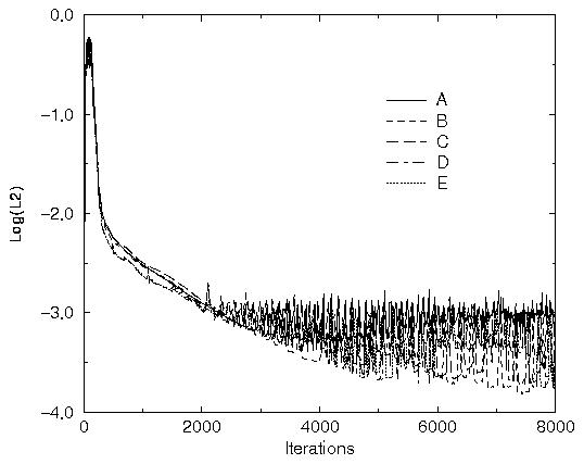
Figure 3. Plot of the L2 solution residual history.
The CFPOST utility can be used to generate the PLOT3D solution files for display in a visualization software package. CFPOST is executed as:
cfpost < cfpost.plot3d.com
The PLOT3D grid file is named run.x and the solution file is named run.q. The file is unformatted, whole, 3D, and multi-zone.
The CFPOST utility can be used to list out and plot the static temperature, pressure, density along the ramp (J1) surface. CFPOST is executed as:
cfpost < cfpost.tpr.com
where the file cfpost.tpr.com is a command file containing the inputs for CFPOST. A GENPLOT file named tpr.gen is created containing the temperature, pressure, and density along the ramp as a function of the x-coordinate. The temperature and pressure were then copied into XY plot files. Table 6 lists all these files for each of the run. Figs. 4 and 5 plot the temperature and pressure distributions for each of the runs.
| Run | Tpr GENPLOT | T-vs-X | p-vs-X | u-vs-y |
|---|---|---|---|---|
| A | tpr.A.gen | T.A.d | p.A.d | u.A.d |
| B | tpr.B.gen | T.B.d | p.B.d | u.B.d |
| C | tpr.C.gen | T.C.d | p.C.d | u.C.d |
| D | tpr.D.gen | T.D.d | p.D.d | u.D.d |
| E | tpr.E.gen | T.E.d | p.E.d | u.E.d |
| F | tpr.F.gen | T.F.d | p.F.d | u.F.d |
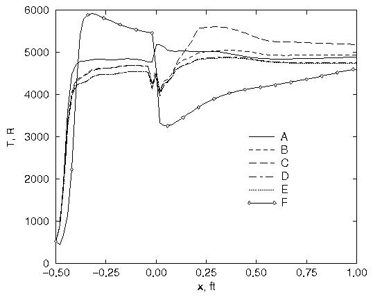
Figure 4. The plots of the temperature distributions along
the ramp.
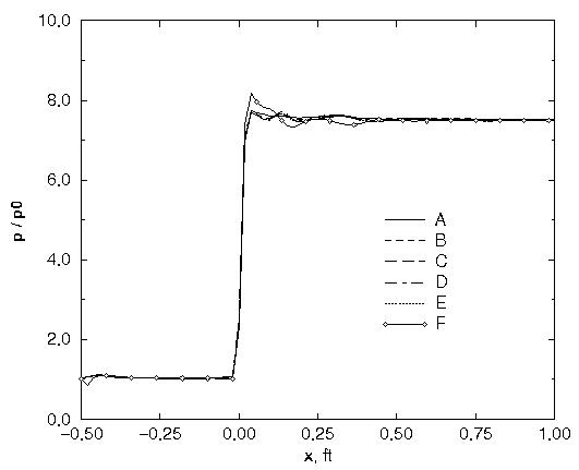
Figure 5. The plots of the pressure distributions along
the ramp.
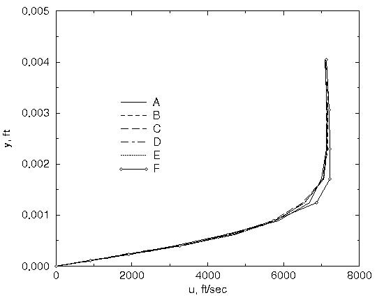
Figure 6. The plots of the u-velocity through the boundary
layer at the end of the ramp.
No analytical or experimental data is available for this study. One observation is that the gas models predict a similar variations for temperature and pressure on the ramp. This indicates that perhaps the high-temperature effects are minimal for this case. The temperature distributions from the PNS run (F) show a questionable result. Note that for the PNS run (F), the pressure does not "see" the ramp until it is at the ramp; whereas the time-dependent computations allow upstream travelling pressure waves in the subsonic portion of the boundary layer.
Other than the sensitivity due to the gas model, no sensitivity studies were performed for this study.
The computations were performed on a Silicon Graphics Octane 2 workstation with 2 600 IP30 MIPS R14000 Processors. Only one processor was used for these computations. The CPU times for the each run is summarized in Table 3 above.
No references available for this study.
This case was created on April 11, 2003 by John W. Slater, who may be contacted at:
NASA Glenn Research Center, MS 86-7
21000 Brookpark Road
Brook Park, Ohio 44135
Phone: (216) 433-8513
e-mail: John.W.Slater@nasa.gov