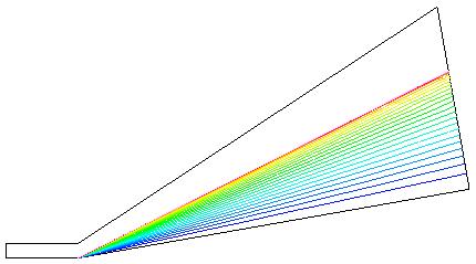
Figure 1. Mach number contours for inviscid Mach 2.35 flow past a 10 degree cone.
Figure 1. Mach number contours for inviscid Mach 2.35 flow
past a 10 degree cone.
This verification case involves the steady, inviscid, adiabatic Mach 2.35 flow over a cone with a semi-vertex angle of 10 degrees. The flow is a classic conical flowfield with an attached shock at the apex of the cone with conical rays of constant properties eminating from the apex. The simulations available here use the structured grid solver of the Wind-US code (version 3.139). The CFD simulation results are compared to results from theoretical supersonic cone flow. Results are also provided from earlier CFD simulations using the NPARC code and an earlier version of the WIND code.
The freestream conditions are presented in Table 1. These conditions correspond to a Reynolds number of 2.5 million / ft, which is a typical operating point of the NASA Glenn 10x10 wind tunnel.
| Mach | Pressure (psia) | Temperature (R) | Angle-of-Attack (deg) | Angle-of-Sideslip (deg) |
|---|---|---|---|---|
| 2.35 | 11.79 | 550.0 | 0.0 | 0.0 |
The geometry is a cone with a semi-vertex angle of 10 degrees and a length of approximately 1.0 ft.
An analytic solution for the inviscid, supersonic, steady, adiabatic flow over a cone is available through the Taylor-Maccoll differential equation as described in most compressible flow textbooks. The program HAP provided as part of the text book "Hypersonic Airbreathing Propulsion" by W.H. Heiser and D.T. Pratt solves this equation for the conditions just after the conical shock and on the cone surface. The subscript 1 refers to the freestream conditions. The subscript 2 refers to the conditions behind the shock. The subscript 3 refers to the conditions one the surface of the cone. The angle of the shock is 27.1843 degrees.
| Property | 2 | 3 |
|---|---|---|
| M | 2.2677 | 2.1469 |
| p / p1 | 1.1781 | 1.4234 |
| T / T1 | 1.0481 | 1.1063 |
| rho / rho1 | 1.1240 | 1.2867 |
| pt / pt1 | 1.0 | 1.0 |
| Tt / Tt1 | 1.0 | 1.0 |
Since the flow is supersonic, the inflow boundary I1 of the domain starts - 0.2 ft ahead of the apex of the cone and flow conditions are FROZEN. The outflow boundary IMAX is at approximately 1.0 ft with supersonic outflow, and so, is specified as an OUTFLOW boundary with extrapolation. The J1 boundary contains the axis-of-symmetry and the cone surface and is specified as an INVISCID WALL. The JMAX boundary is the supersonic freestream, and so, is specified as FROZEN. For three-dimensional computations, the K1 and KMAX boundaries are specified as REFLECTION planes.
The grids for the axisymmetric and three-dimensional domains are cone10.x.axi.fmt and cone10.x.3D.fmt, respectively, and are in Plot3d format (formatted, multi-zone, 3D, whole, double-precision). These are converted to the common grid file format as cone10.WindUS3.axi.cgd and cone10.WindUS3.3D.cgd, respectively. The grid size of the three-dimensional grid is (121,81,5). The axisymmetric grid uses only one K plane for the planar axisymmetric computations.
The boundary conditions are implemented through GMAN as
gman < gman.axi.com
gman < gman.3D.com
The initial flow conditions are the freestream conditions. WIND by default creates this.
The computation is performed using the time-marching capabilities of Wind-US to march to a steady-state (time asymptotic) solution. Local time stepping is used at each iteration. The time-marching is performed until convergence criteria is achieved. Both planar axisymmetric and three-dimensional domains are used for the Wind-US simulations.
The input data file for the planar axisymmetric Wind-US simulation was cone10.WindUS3.axi.dat. A 5 degree axisymmetric extent was specified. The CFL number used was 0.5, although a higher CFL number could have been used.
The input data file for the three-dimensional Wind-US simulation was cone10.WindUS3.3D.dat. A CFL number of 1.5 was used. Grid sequencing was used to enhance the iterative converge through 3 grid sizes each twice as fine as the previous. Each level was brought to iterative convergence over 300 cycles.
The computations were performed using Wind-US. Table 3 lists the input and output files.
| File | Wind-US 3.0 (Axi) | Wind-US 3.0 (3D) |
|---|---|---|
| Grid | cone10.WindUS3.axi.cgd | cone10.WindUS3.3D.cgd |
| Input Data File | cone10.WindUS3.axi.dat | cone10.WindUS3.3D.dat |
| Solution | cone10.WindUS3.axi.cfl | cone10.WindUS3.3D.cfl |
| List / Residual | cone10.WindUS3.axi.lis | cone10.WindUS3.3D.lis |
The residual information was read from the WIND list files using the RESPLT utility and plotted using CFPOST,
resplt < resplt.nsl2.com
cfpost < cfpost.nsl2.com
The convergence was checked by acknowledging that the L2 norm of the residuals had leveled off and then by the constancy of the average Mach number on the cone surface.
The CFPOST utility was used to obtain information from the solution.
Flowfield Mach Number Contours. The Mach number contours for the flow field can be generated by
cfpost < cfpost.mach.com
Properties at IMAX. The properties at IMAX are output to the GENPLOT file IMAX.gen by
cfpost < cfpost.IMAX.com
Properties at J1. The properties along J1, which includes the cone surface, are output to the GENPLOT file J1.gen by
cfpost < cfpost.J1.com
The Mach number on the cone surface can be output to the GENPLOT file machcone.gen by
cfpost < cfpost.machcone.com
The average Mach number (or other average property) can be computed using the Fortran program mavg.f. It simply sums up the values after x of 0.2 and averages them. The values should be fairly constant.
A comparison of the properties on the cone surface are provided below in Table 4. The results for the Wind-US simulations are listed along with the results from theory and earlier CFD simulations with the WIND and NPARC codes. All of the CFD simulations indicate similar differences with respect to the theory.
| Computation | M3 | Error% | p3/p1 | Error% | T3/T1 | Error% |
|---|---|---|---|---|---|---|
| Theory | 2.1469 | - | 1.4234 | - | 1.1063 | - |
| WIND-AXI | 2.1469 | 0.0000 | 1.3741 | -3.4635 | 1.0951 | -1.0124 |
| WIND-3D | 2.1467 | -0.0074 | 1.3741 | -3.4635 | 1.0951 | -1.0124 |
| NPARC-AXI | 2.1467 | -0.0074 | 1.3741 | -3.4635 | 1.0951 | -1.0124 |
| Wind-US 3.0 (axi) | 2.1468 | -0.0047 | 1.3740 | -3.4706 | 1.0951 | -1.0124 |
| Wind-US 3.0 (3D) | 2.1468 | -0.0047 | 1.3741 | -3.4635 | 1.0951 | -1.0124 |
A grid convergence study was performed using the 3 levels of grids of the WIND axisymmetric computations. The Fortran program verify.f90 is used to perform the computations of the grid convergence study. The output is printed below. The results indicted that the solutions are well within the asymptotic range.
 --- VERIFY: Performs verification calculations ---

 Number of data sets read =  3

      Grid Size     Quantity

      1.000000      2.146783
      2.000000      2.146728
      4.000000      2.146115

 Order of convergence using first three finest grid
 and assuming constant grid refinement (Eqn. 5.10.6.1)
 Order of Convergence, p =  3.47636485

 Richardson Extrapolation: Use above order of convergence
 and first and second finest grids (Eqn. 5.4.1)
 Estimate to zero grid value, f_exact =  2.1467886

 Grid Convergence Index on fine grids. Uses p from above.
 Factor of Safety =  1.25

   Grid     Refinement
   Step      Ratio, r       GCI(%)
   1  2      2.000000      0.000680
   2  3      2.000000      0.007564

 Checking for asymptotic range using Eqn. 5.10.5.2.
 A ratio of 1.0 indicates asymptotic range.

  Grid Range    Ratio
  12 23      1.000000

 --- End of VERIFY ---
Anderson, J.D., Modern Compressible Flow , McGraw Hill Inc., New York, 1982.
Heiser, W.H. and D.T. Pratt, Hypersonic Airbreathing Propulsion, AIAA Education Series, Washington, D.C., 1994.
Questions or comments about this case can be sent be emailed to John W. Slater,
NASA John H. Glenn Research Center, MS 5-12
21000 Brookpark Road
Cleveland, Ohio 44135
Phone: (216) 433-8513
e-mail: John.W.Slater@nasa.gov