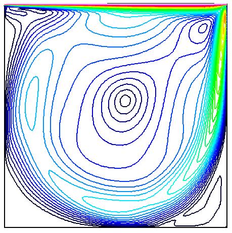
Figure 1. The Mach number contours for the driven
cavity run C with Reynolds number of 3200.
Figure 1. The Mach number contours for the driven
cavity run C with Reynolds number of 3200.
All of the archive files of this validation case are available in the Unix compressed tar file cavity.tar.Z. The files can then be accessed by the commands
uncompress cavity.tar.Z
tar -xvof cavity.tar
The grid used was a simple non-clustered rectangular grid with 65x65 points for Re = 100 (run A) and 128x128 for runs B and C.
| Topology: | Structured, multi-block |
| Number of Blocks: | 1 |

Figure 2. A plot of the example grid for the
driven cavity case.
Table 1 lists the names of the common grid files (*.cgd) and the PLOT3D grid files for the grids. The PLOT3D files are three-dimensional, whole, single-block and unformatted.
| Run | Reynolds Number | Grid Size | CGD File | PLOT3D Grid File |
|---|---|---|---|---|
| A | 100 | 65 x 65 | cavity.A.cgd | cavity.A.x.bin |
| B | 400 | 128 x 128 | cavity.B.cgd | cavity.B.x.bin |
| C | 3200 | 128 x 128 | cavity.C.cgd | cavity.C.x.bin |
GMAN is executed for each run in following manner,
gman < gman.A.com
gman < gman.B.com
gman < gman.C.com
The flowfields for the runs are intialized according to the conditions specified in the FREESTREAM keyword in the input data files (*.dat). These conditions are listed in Table 2. The static pressure varies for each run to achieve the desired Reynolds number. How the pressure is computed is discussed below.
| Mach number | Temperature(R) | Angle-of-Attack (deg) |
|---|---|---|
| 0.05 | 460.0 | 0.0 |
The computations were performed using the time-marching capabilities of WIND to approach the steady-state flow starting from the freestream conditions.
Table 3 below lists the name of the input data files for the three runs. The runs used the default input values for WIND. The computations were performed for a set number of iterations until that the convergence histories leveled out.
For all of the runs, we assume the gas in the box is ideal air (R = 1714.48 ft^2/(s^2*deg R) and ratio of specific heats = 1.4). The freestream conditions involved a Mach number of 0.05 and a static temperature 460 degrees Rankine. These (arbitrary) choices resulted in a freestream velocity of 52.56 ft/s, which was used as the velocity of the upper boundary wall in order for the freestream Reynolds number to be the same as the Reynolds number based on the wall velocity.
Assuming a viscosity determined by Sutherland's law and using a reference length of 1 inch, we get the following relation between Re and freestream pressure:
p_infty = (4.250e-04 lbf/in^2)*Re_infty
Thus the freestream pressure is used as a parameter which is chosen to reflect a desired Reynolds number (other parameters listed as well).
| Run | Static pressure (psia) |
|---|---|
| A | 0.0425 |
| B | 0.17 |
| C | 1.3 |
| Run | Reynolds Number | Input Data File | CFL Number | Iterations | CPU Time (sec) |
|---|---|---|---|---|---|
| A | 100 | cavity.A.dat | 0.5 | 25000 | 29677.96 |
| B | 400 | cavity.B.dat | 1.5 | 11193 | - |
| C | 3200 | cavity.C.dat | 1.5 | 30000 | 162186.06 |
For each of the runs, WIND produces a listing file (.lis) and a solution file (.cfl). Note the list file for run B end prematurely, and so, the CPU times are not available. The files are listed below in Table 5.
| Run | Reynolds Number | List File | L2 Residual | CFL File | PLOT3D Solution |
|---|---|---|---|---|---|
| A | 100 | cavity.A.lis | cavity.A.resl2.gen | cavity.A.cfl | cavity.A.q.bin |
| B | 400 | cavity.B.lis | cavity.B.resl2.gen | cavity.B.cfl | cavity.B.q.bin |
| C | 3200 | cavity.C.lis | cavity.C.resl2.gen | cavity.C.cfl | cavity.C.q.bin |
The convergence histories of the L2 residual for each run can be obtained from the list files (*.lis), listed in Table 5 above, using the utility RESPLT. The GENPLOT files created can be viewed with CFPOST using the command
plot data cavity.A.resl2.gen
These GENPLOT files are listed in Table 5 above. Figure 3 below shows these convergence histories.
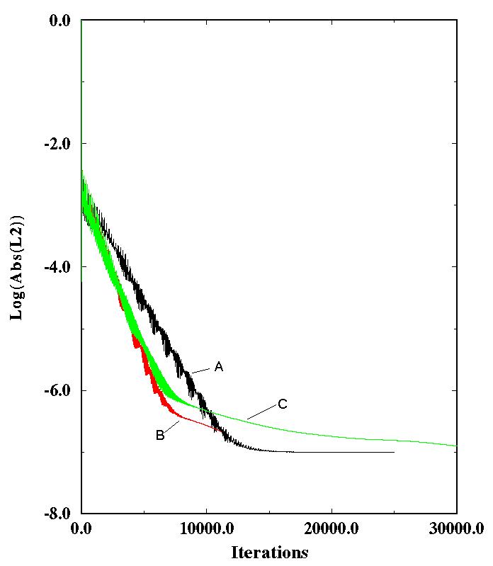
Figure 3. The plot of the convergence history for the
WIND computations of flow in the driven cavity.
The CFPOST utility was used to generate the PLOT3D grid and solution files for each run. The PLOT3D grid and solution files are listed in Tables 1 and 5, respectively.,
cfpost < cfpost.A.com
cfpost < cfpost.B.com
cfpost < cfpost.C.com
A cursory comparison of these results was made with results from Ghia, Ghia, and Shin (Journal of Computational Physics, Vol. 48, pp. 387-411, 1982). Using an eyeball comparison, WIND appears to produce very similar solution results.
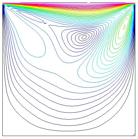
Figure 4. The plot of the mach number contours for the
driven cavity with a Reynolds number of 100.
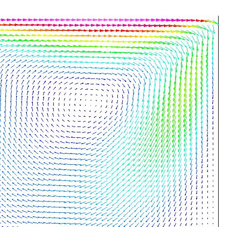
Figure 5. The plot of the velocity vectors colored by
the Mach number near the upper right corner for the
driven cavity with a Reynolds number of 100.
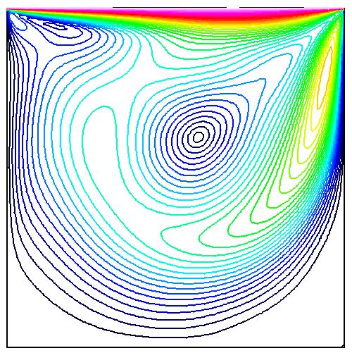
Figure 6. The plot of the mach number contours for the
driven cavity with a Reynolds number of 400.
These runs were performed on a Silicon Graphics Indigo-2 with a IP22 processor running IRIX 5.3. The CPU times are listed above in Table 4. Note that the CPU time for run B was not available because the list file is incomplete.
Ghia, Ghia, and Shin, Journal of Computational Physics, Vol. 48, pp. 387-411, 1982.