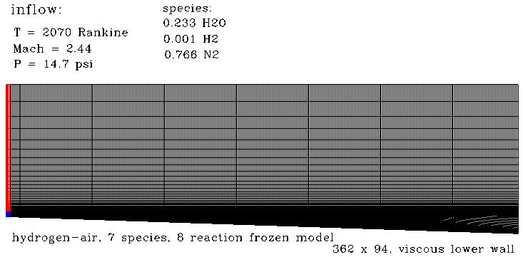
Figure 1: Schematic of the dual-stream mixing duct and inflow conditions.
Figure 1: Schematic of the dual-stream mixing duct and inflow conditions.
This study focuses on a frozen, hydrogen-air mixing occuring within a non-constant area channel with two separate inflow streams. The upper (shown in red in Figure 1) consists of a vitiated air mixture of H2, H2O and N2, and the lower (shown in blue in Figure 1) of pure hydrogen. Species mass fraction values and turbulence modeling effects downstream of the inflow are investigated. The WIND (version 5.116 ALPHA) results are compared to experimental and numerical results for Case 2 in the reference paper. All calculations presented here use a multi-zone two-dimensional grid.
A 362 x 94 mesh was generated to model the channel region from 0 to 14 inches downstream. The channel is 14 inches long and 3.66 inches tall at the inflow. The lower viscous wall was clustered to y+ values of 1, and is slanted slightly downward to account for the boundary layer development. A small "cap" was added to the beginning of the duct to aid application of different boundary conditions at the inflow, eliminating zonal boundaries running axially through the flowfield. Zonal boundaries are known to cause problems when running turbulence models. From Figures 2 and 3, it is seen that the 94 x 181 grid was adequate to predict mixing.
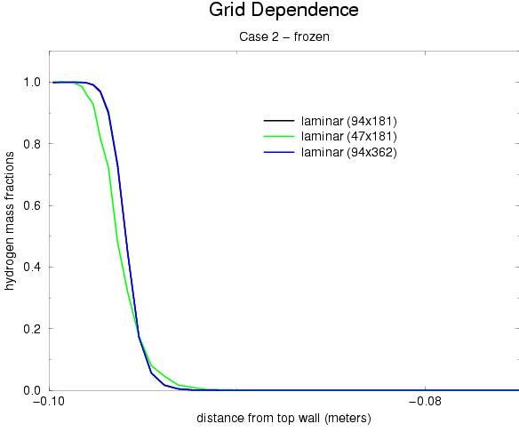
Figure 2: Grid Dependence: laminar model
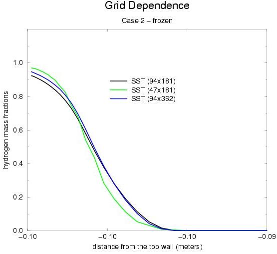
Figure 3: Grid Dependence: Mentor SST model
This grid is provided below in Plot3d (two-dimensional, multiple-grid, unformatted, whole) and common file format. The coordinates in both files are in units of inches
| Plot3D | Common Grid |
| case2.xyz | case2.cgd |
Two separate streams exist at the inflow. The duct is 3.66 inches tall of which 0.152 inches is dedicated to the hydrogen stream (indicated in blue in Figure 1). The vitiated air inflow is represented by red in Figure 1. The upper region (red) was set to static conditions of 2070 Rankine, a pressure of 14.7 psi, and Mach number 2.44. In addition, species mass fractions were set to 0.233 for H2O, 0.001 for H2, and 0.766 for N2 (all others set to zero). The hydrogen stream (indicated by blue in Figure 1) was set to static conditions of 540 Rankine, 14.7 psi, and Mach number of 1. In this case, the chemistry file h2air-7sp-std-15k.chm was used for the frozen calculations. The crossflow CFL and TVD factors were set to a value of 1. The laminar, PDT, Chien k-e, Spalart-Allmaras, and Mentor SST turbulence models were applied.
The frozen boundary condition was used for the vitiated air inflow, arbitrary inflow for the hydrogen stream, inviscid or wall slip BC employed for the upper wall, viscous for the lower wall, and the outflow boundary condition was used at the exit (forcing extrapolation of the pressure).
The computation is performed using the time-marching capabilities of WIND to march to a steady-state (time asymptotic) solution. Local time stepping is used at each iteration. The time-marching is performed until the convergence criteria is achieved. The solution was started laminar at a CFL number of 0.1. The turbulence models were then switched on the CFL number was ramped up to 0.8 for the remainder of the run. The SST case ran for a total of 81,358 iterations.
The input data file for WIND is case2.dat.
The WIND flow solver is run, creating the following output files:
| Plot3D | Common File Solution | List File |
|---|---|---|
| case2.q | case2.cfl | case2.lis.gz |
Convergence information for the SST case can be obtained from the case2.lis.gz file by using the resplt utility program.
Species mass fractions for H2, H2O and N2 at the exit plane (14 inches downstream) were compared to Case 2 in the reference paper for various turbulence models. Plots of species mass fractions vs downstream distance. The paper's results were computed with the NASTD code, a precurser to the WIND code. NASTD predicted a mass fraction value of 1 for hydrogen at the lower wall (the black line) in Figure 4. The WIND SST model predicted about 0.92 (the blue line), followed by Spalart-Allmaras at 0.8 (the green line). Both the k-e and PDT models failed to development an eddy viscosity profile across the mixing layer, and are not shown here. Figures 7 through 12 show various flowfield contours in the x-y plane.
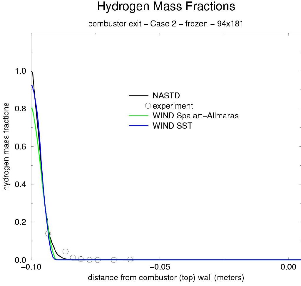
Figure 4: H2 mass fractions at duct exit
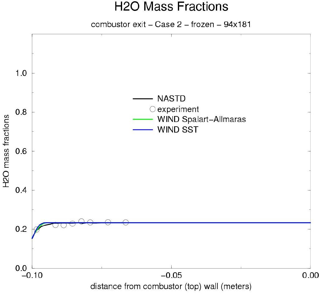
Figure 5: H2O mass fractions at duct exit
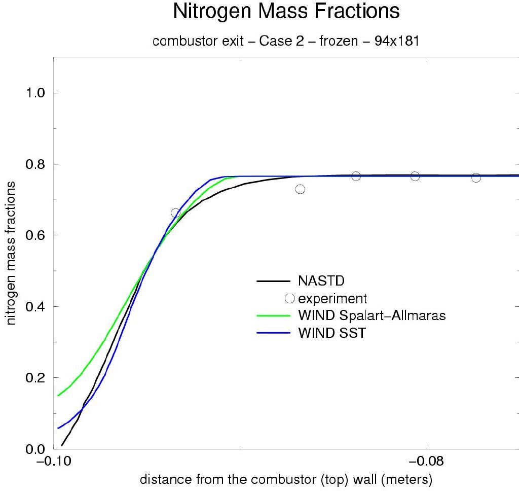
Figure 6: N2 mass fractions at duct exit
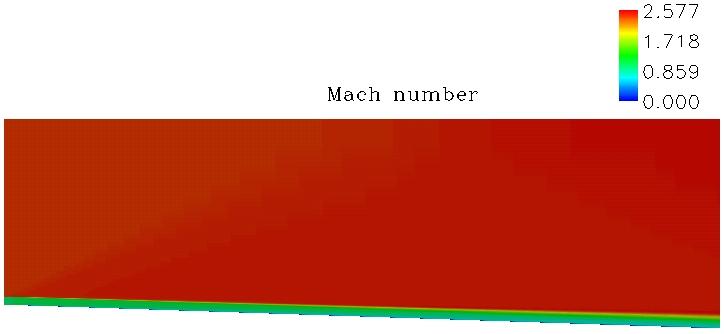
Figure 7: Mach Number contours in the x-y plane.
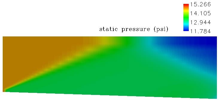
Figure 8: Static pressure contours in the x-y plane.
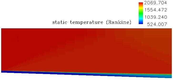
Figure 9: Static Temperature contours in the x-y plane.
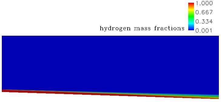
Figure 10: Hydrogen mass fractions contours in the x-y plane.
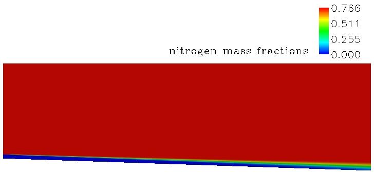
Figure 11: Nitrogen mass fractions contours in the x-y plane.
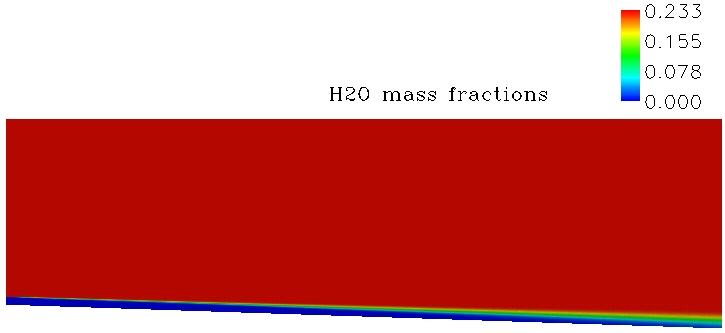
Figure 12: H2O mass fractions contours in the x-y plane.
Mani, M., Bush, R.H., Vogel, P.G., "Implicit Equilibrium and Finite-Rate Chemistry Models For High Speed Flow Applications," AIAA Paper 91-3299-CP, Jan. 1991.
Burrows, M.C., Kurkov, A.P., "Analytical and Experimental Study of Supersonic Combustion of Hydrogen in a Vitiated Airstream, " NASA-TM-X-2828, September 1973.
This case was created on April 19, 2002 by Teryn DalBello, who may be contacted at
NASA Glenn Research Center
21000 Brookpark Road, MS 86-7
Cleveland, Ohio 44111
Phone: (216) 433-8412
e-mail: teryn@grc.nasa.gov