 NPARC Alliance Validation Archive
This study is an example study demonstrating the use of Wind-US to compute axisymmetric, nozzle flow fields.
All of the files associated with this study are available in the compressed tar file axinoz01.tar.gz. The files can then be accessed by the commands
gunzip axinoz01.tar.gz
tar -xvof axinoz01.tar
This grid is available as a Plot3d grid file axinoz.x.fmt (formatted, 3D, multi-zone).
The Plot3d grid file is converted to the common grid file (.cgd) format using the CFCNVT utility. This is done using the command
cfcnvt < cfcnvt.x.com
where the file cfcnvt.x.com is a command input file (standard Fortran input unit). A common grid file named axinoz.cgd is created.
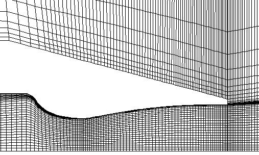
Zone 1 contains the internal flow field of the nozzle. The grid is clustered to the nozzle wall to resolve the boundary layers at the no-slip surface. Zone 2 is exterior to the nozzle. The exterior surfaces of the nozzle are modeled as slip surfaces. Zone 3 is downstream of the nozzle. There is a blunt nozzle lip which is modeled as a slip surface. Fig. 2 shows the grid near the nozzle (note that the grid has been coarsened by half for clarity).
The nozzle inflow boundary is specified as an ARBITRARY INFLOW boundary with total pressure and total temperature specified. The axis-of-symmetry is specified as a INVISCID WALL boundary for this axisymmetric flow computation. The internal surface of the nozzle is specified as a VISCOUS WALL boundary, while the external nozzle surfaces are specified as INVISCID WALL boundaries since the influence of the exterior boundary layer is not considered significant for this analysis. The exterior inflow and farfield boundaries are specified as FREESTREAM boundaries. The exterior outflow boundary is specified as a OUTFLOW boundary.
The boundary conditions are set within the commond grid file axinoz.cgd by using the GMAN utility
gman <gman.com
where the file gman.com is a command input file. The commond grid file axinoz.cgd is updated in the process.
The computation is performed using the time-marching capabilities of Wind-US to march to a steady-state (time asymptotic) solution. Local time stepping is used at each iteration. The time-marching is performed until convergence criteria is achieved.
The flow field initialization is performed within Wind-US. The arbitrary inflow keyword in the input data file axinoz.dat for zone 1 initializes the entire zone to the conditions specified in the arbitrary inflow section. Zones 2 and 3 are initialized to uniform conditions according to the freestream conditions.
The input data file for Wind-US is axinoz.dat. The freestream keyword specifies the ambient conditions. Since Wind-US requires a non-zero Mach number to be specified, a Mach number of 0.05 is used for quiescent conditions. The Spalart-Allmaras turbulence model is specified through the turbulence keyword. The flow is solved with an axisymmetric flow domain through the axisymmetric keyword. The y-coordinate is set to 0.0 and a 5.0 degree angle section is specified. The OUTFLOW boundary condition was used for the outflow boundary of zone 3. Thus, the downstream pressure keyword is used to set the static pressure at that boundary as the freestream value. The arbitrary inflow keyword is used to set the plenum conditions at the nozzle inflow. The loads keyword is used to output the mass flow at the nozzle exit.
The Wind-US flow solver is run using the wind script,
wind -runinplace -dat axinoz -mp -parallel
The list file is axinoz.lis and contains the output from the computation and lists the residual information for all of the iterations. The flow data file is axinoz.cfl and contains the final solution.
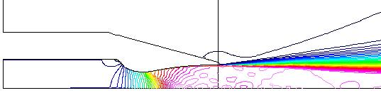
Figure 3 shows the Mach number contours for the entire flow domain.
Information on the convergence properties of the solution can be obtained from the list file axinoz.lis using the RESPLT utility. It can then be plotted using CFPOST,
resplt < resplt.nsl2.com
cfpost < cfpost.nsl2.com
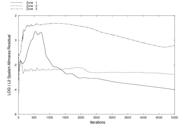
The file resplt.nsl2.com is a command file containing the inputs for RESPLT to output the file nsl2.gen containing the L2 residual history of the Navier-Stokes equations.
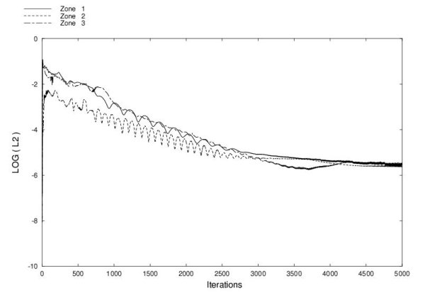
The convergence of the Spalart-Allmaras turbulence model can be examined and plotted using RESPLT and CFPOST,
resplt < resplt.sal2.com
cfpost < cfpost.sal2.com
The file resplt.sal2.com is a command file containing the inputs for RESPLT to output the file sal2.gen containing the L2 residual history of the turbulent eddy viscosty equation solved by the Spalart-Allmaras model.
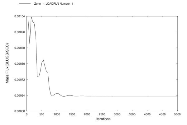
Another measure of convergence is the mass flow out of the nozzle. Within the input data file axinoz.dat, the loads keyword indicated that the mass flux out of the nozzle was to be output to the output list file axinoz.lis. The history of this mass flux can be examined using RESPLT and plotted using CFPOST,
resplt < resplt.mass.com
cfpost < cfpost.mass.com
The file resplt.mass.com is a command file containing the inputs for RESPLT to output the file mass.gen containing the iteration history of the mass flux out of the nozzle.
PLOT3D Solution File. The PLOT3D solution file (formatted, multi-zone) named axinoz.q.fmt can be generated using the CFPOST utility,
cfpost < cfpost.plot3d.q.com
Inflow Conditions. The flow conditions at the nozzle inflow can be written out to check if the total pressure and total temperature were held fixed. This is done using the CFPOST utility,
cfpost < cfpost.inflow.com
The file cfpost.inflow.com is a command file which writes out the data to the GENPLOT file inflow.gen.
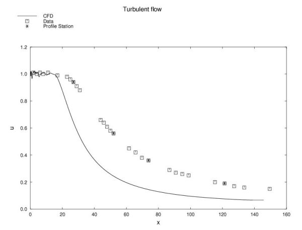
Axial Centerline Velocity. The axial velocity along the centerline can be output using the CFPOST utility,
cfpost < cfpost.axial.com
The file cfpost.axial.com is a command file which writes out the data to the GENPLOT file axial.u.gen. The axial velocity is scaled by the reference axial velocity (1765 ft/sec). The axial distance is the distance from the nozzle exit scaled by the nozzle exit radius (0.5035 in). Figure 7 compares the computed axial velocity to that measured from the experiment and contained in the plot file axial.u.ex.gen.
Velocity Profiles. The velocity profiles in the radial direction at several axial stations downstream of the nozzle exit and through the jet were examined and compared to the experimental values. Comparisons were made at five axial stations: 0.0, 26.93, 51.96, 73.80, and 121.30, which are distances from the nozzle exit nondimensionalized by the nozzle exit radius. These stations correspond to grid lines with an i-index of 1, 112, 126, 134, and 145, respectively. The velocities at these stations were obtained using CFPOST
cfpost < cfpost.prof001.com
cfpost < cfpost.prof112.com
cfpost < cfpost.prof126.com
cfpost < cfpost.prof134.com
cfpost < cfpost.prof145.com
This produced the following GENPLOT files prof001.gen, prof112.gen, prof126.gen, prof134.gen, and prof145.gen.
The cooresponding experimental profile data for these stations were taken from the file profile.dat and put into the plot files files prof001.ex.gen, prof112.ex.gen, prof126.ex.gen, prof134.ex.gen, and prof145.ex.gen.
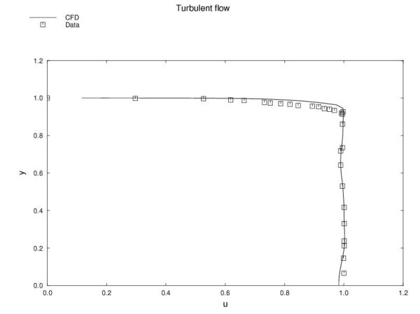
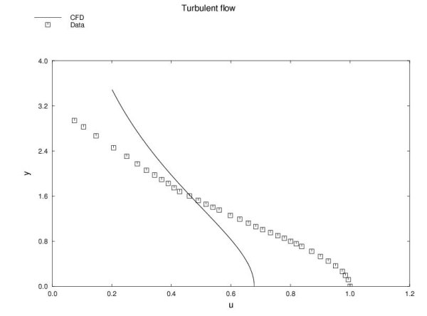
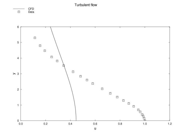
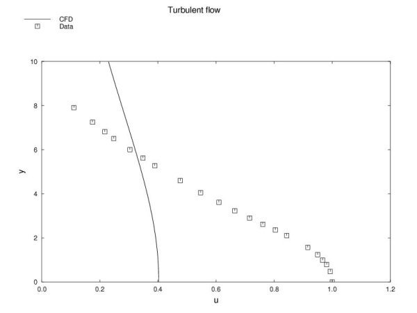
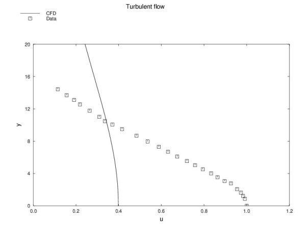
Comparisons are made with measured velocity distributions along the centerline and at five axial stations which span the region prior to closure of the inviscid core to the incompressible self-similar farfield. From Figures 7-12, it appears that the jet is spread out at a greater rate than predicted in the experiment. It is felt that the accuracy of this computation is sensitive to the turbulence modeling.
Eggers, J.M. "Velocity Profiles and Eddy Viscosity Distributions Downstream of a Mach 2.22 Nozzle Exhausting to Quiescent Air," NASA TN D-3601, September 1966. [PDF]
This case was updated on May 30, 2008 by John W. Slater, who may be contacted at
NASA Glenn Research Center, MS 5-12
21000 Brookpark Road
Cleveland, Ohio 44111
Phone: (216) 433-8513
e-mail: John.W.Slater@nasa.gov