NPARC Alliance Validation Archive
Validation Home >
Wind-US Tutorial for the M2129 S-duct
Wind-US Tutorial for the M2129 S-duct
by Stan Mohler, Jr.
QSS Group, Inc. at NASA Glenn Research Center
Introduction
This tutorial shows how to do most of the CFD process using unstructured grids with
the NPARC Alliance
Wind-US CFD flow solver. The particular case used here is the M2129
S-duct with high subsonic flow and no vane effectors. This case and some variations
are discussed in a technical paper available on-line:
Wind-US Flow Calculations for the M2129 S-Duct
Using Structured and Unstructured Grids
The following steps are covered in this tutorial:
- Generate the grid - some brief remarks only
- Start MADCAP, and open the CGD file
- Make the surface segments visible
- Reorient the surfaces
- Tell MADCAP that you will assign BC's to this CGD file
- Assign BC's to surfaces
- Quit MADCAP
- Run the usplit-hybrid utility to automatically split the one zone into many
- Create the Wind-US .dat input file
- Run Wind-US
- Post-process using RESPLT and CFPOST
- Further post-processing
Generate the grid
This tutorial will not show how to generate the grids. Rather, it assumes you
are starting with a CGD file containing a single unstructured zone for the
baseline M2129 S-duct.
Unstructured grids for Wind-US can be generated with any grid generator that
can export the grids in unstructured CGD format or
else AFLR3 format (which MADCAP can import and then export as CGD). Currently,
the following grid generators should do this:
-
Gridgen v.15.04 or above
-
ICEM Tetra/Prism
-
SolidMesh + AFLR3
-
Boeing's proprietary version of MADCAP + AFLR3
If you know of additional packages, please let us know so that we may update
this list.
Now do the following:
-
Identify a directory on your computer to work in, and go there.
Note: Make sure the path is short enough such that the path plus any filename
is no more than 80 characters long (due to limitations in MADCAP and the
usplit-hybrid utility).
-
Download the file
M2129-u-base-0-1zone.cgd.gz.
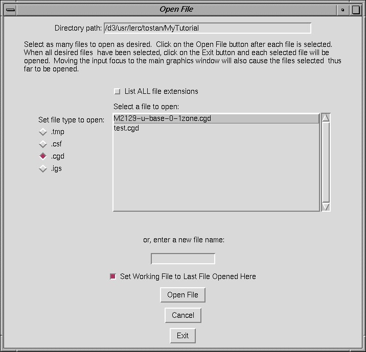
Start MADCAP, and open the CGD file
-
Start MADCAP by typing madcap.
-
Click File -> Open.
-
Select file type as ".cgd".
-
Select the file to open from the list.
-
Check the "Set Working File to Last File Opened Here" box.
The window should now look like so:
-
Click the "Open File" button.
-
Click "Exit."
Make the surface segments visible
-
Find the list of zones on the left side. Only "ZONE 1" is listed.
-
Click on "ZONE 1" with the MIDDLE mouse button.
-
Click on "BOUNDARY SURFACES" with the MIDDLE mouse button.
-
Notice the list of "USURF" surface segments.
-
Make the USURF surface segments visible by clicking on each
"USURF = XXXX" with the LEFT mouse button.
-
The USURF numbers were generated by the grid generator. Notice that there
are a few pairs of USURFs associated with each other. For example,
USURF 15, consisting of triangles, is adjacent to USURF 10015, consisting
of recangles for viscous packing near the wall.
-
Notice that you can repeat Step 5 to toggle each USURF on and off.
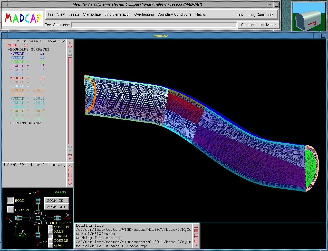
Reorient the surfaces
-
Press the 'M' key to toggle on the "Mouse Transformation Mode". Note the
words "MOUSE TRANSFORMATION MODE" in the graphics window. This
mode allows you to reorient the geometry by dragging the mouse across
the graphics window.
-
Press 'M' again just to see the toggling action.
-
Press 'M' a third time, to leave you in mouse transformation mode.
-
Rotate the geometry: move the mouse pointer into the graphics window, hold
down the LEFT mouse button, and drag the mouse upwards and to the left.
-
Zoom in by holding down the RIGHT mouse button and dragging the mouse
towards you.
-
Try translating using the MIDDLE mouse button.
-
Zoom way out.
-
Press 'M', to toggle off mouse transformation mode.
-
Put the mouse pointer on some piece of geometry where you'd like to zoom in.
-
Now zoom in another way: press and hold down the MIDDLE mouse button while
dragging in any direction. Notice the zoom box you are creating.
When the zoom box just enveloppes the surfaces, let go of the mouse
button.
-
Pick a new center of rotation by MIDDLE clicking at any point on the
surfaces. However BE CAREFUL to keep the mouse very still! The
slightest movement of the mouse will create a tiny zoom box. If you
find you have zoomed way in, just zoom back out as in step 5: press 'M',
then hold down the right mouse button and push the mouse away from you,
let go, and hit 'M' again.
MADCAP should now look something like the following:
Tell MADCAP that you will assign BC's to this CGD file
-
On the main menu, click Boundary Conditions -> Set Boundary Condition File.
-
Click on the CGD file.
-
Press "Set BC File".
Assign BC's to surfaces
-
Zoom in to the upstream end of the S-duct (step 10 above).
-
Turn off the plane-of-symmetry surfaces, to get them out of the way. One
way is to try toggling surfaces on and off from the list. You'll find
there are 12: USURF numbers 15-20 and 10015-10020.
-
Left-click at any point on any of the visible surfaces. Notice the
report that appears in the lower right corner of the graphics window
giving the surface name (i.e., USURF number), the boundary condition at
that point (currently set to UNKNOWN), and some other information.
-
Left-click on the two inflow surfaces and note their names. They are
called USURF 13 and USURF 10013.
-
On the main menu, click Boundary Conditions -> Set Boundary Condition Region.
-
Click "ZONE 1:".
-
Click "U13".
-
Click "Set Boundary".
-
Click Boundary Conditions -> Set Boundary Condition.
-
From the column on the right, click on "ARBITRARY INFLOW".
-
Click "Set BC's".
-
Click Boundary Conditions -> Update Boundarya Conditions.
-
To verify that you have assigned the inflow BC, left-click on any point
of USURF 13 in the graphics window. The report should should say,
"Boundary Condition = 7: ARBITRARY INFLOW".
-
In like manner, repeat steps 1-13 to assign BC's to the rest of the
surface segments. Use Outflow, Viscous Wall, and Reflection BC's. Reflection BC's go on the plane of symmetry.
Quit MADCAP
-
Click File -> Quit.
-
Click one of the two "Yes" buttons.
Run the usplit-hybrid utility to automatically split the one zone into
many
-
Shorten the name of the CGD file: copy it to "1zone.cgd". This is because
usplit-hybrid has trouble if the path and file name are too long.
-
Start usplit-hybrid by typing usplit-hybrid.
-
When prompted, type in the name of the CGD file: 1zone.cgd
-
Type in a name for the new, multi-zone CGD file: 5zones.cgd
-
When prompted, enter the number of zones to create: 5
-
usplit-hybrid prints lots of output, and then finishes.
-
Verify that a new CGD file was created named 5zones.cgd.
-
Rename 5zones.cgd to M2129-u-base-0-5zones.cgd .
-
This file has 5 zones. The BC's you assigned previously have been carried
over into this new CGD file. You can verify this by examining
the new file with MADCAP. In addition, you will discover a bunch of
new, crinkly surfaces at the zone boundaries. Points on these surfaces
have a coupled BC assigned to them by usplit-hybrid. They have negative
USURF numbers.
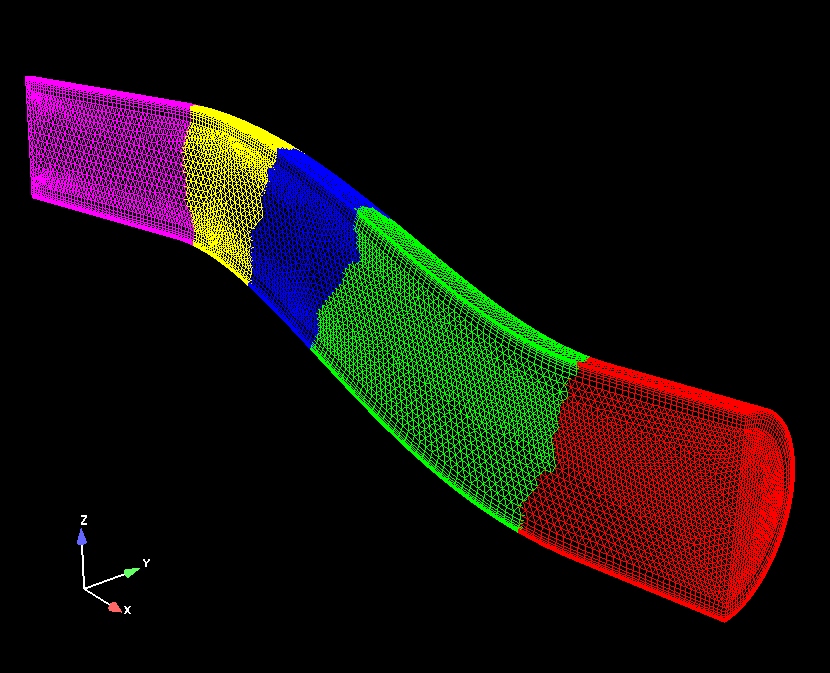
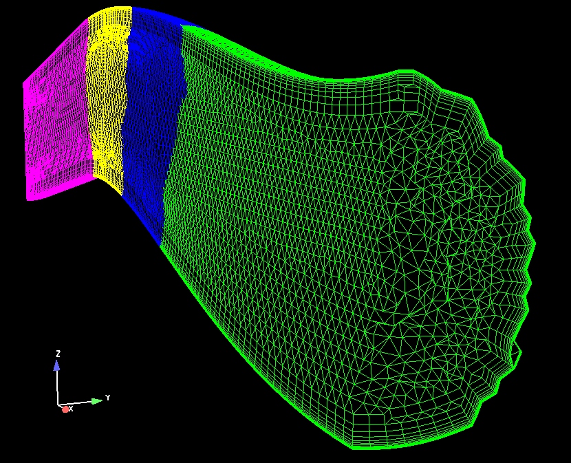
The 5 zones look like so:
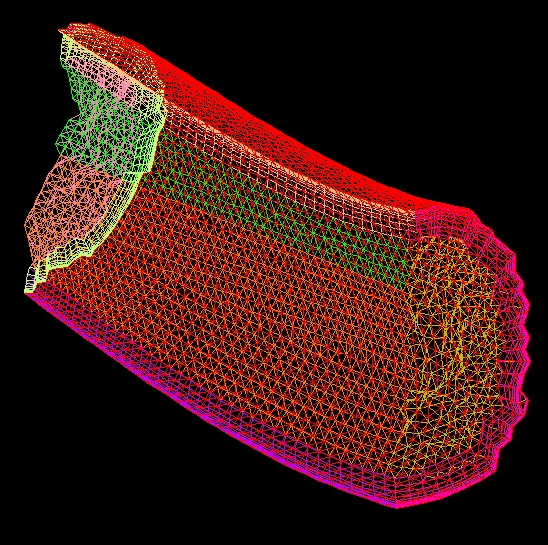
A crinkly zone boundary looks as follows:
In MADCAP, one of the new zones would look as below.
The newly created
crinkly surfaces are listed with negative USURF numbers.
Create the Wind-US .dat input file
-
Get the file
M2129-u-base-0-5zones.dat .
-
Study the comments in the file.
Run Wind-US
-
Start Wind-US as you have always started up the WIND code. Use the input
files listed here:
M2129-u-base-0-5zones.cgd.gz
M2129-u-base-0-5zones.dat
M2129-u-base-0-5zones.mpc
-
Watch the .lis output file as it grows. It reports your inputs, and
then proceeds to print the convergence history as Wind-US runs.
-
The run will stop after 12000 iterations.
- Note the creation of the CFL and .tda files.
- Here is the CFL file and an abbreviated version of the LIS file
produced by my own run:
M2129-u-base-0-5zones.lis.ABBREV
M2129-u-base-0-5zones.cfl.gz
Post-process using RESPLT and CFPOST
Run the following command lines:
-
Get the file resplt.in .
-
Run RESPLT to create file resplt.gen which will hold L2 history data:
resplt < resplt.in
-
Get the file cfpost.res.com .
-
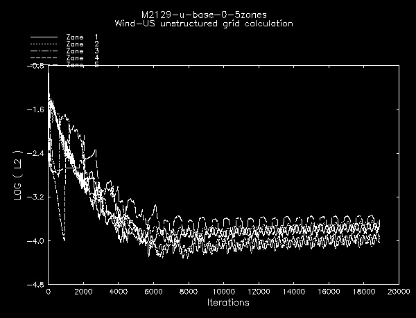
Run CFPOST to display the L2 history:
cfpost < cfpost.res.com
You will see something like the following plot:
-
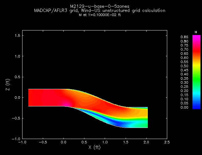
Get the file cfpost.com .
-
Run CFPOST to display the flow field:
cfpost < cfpost.com
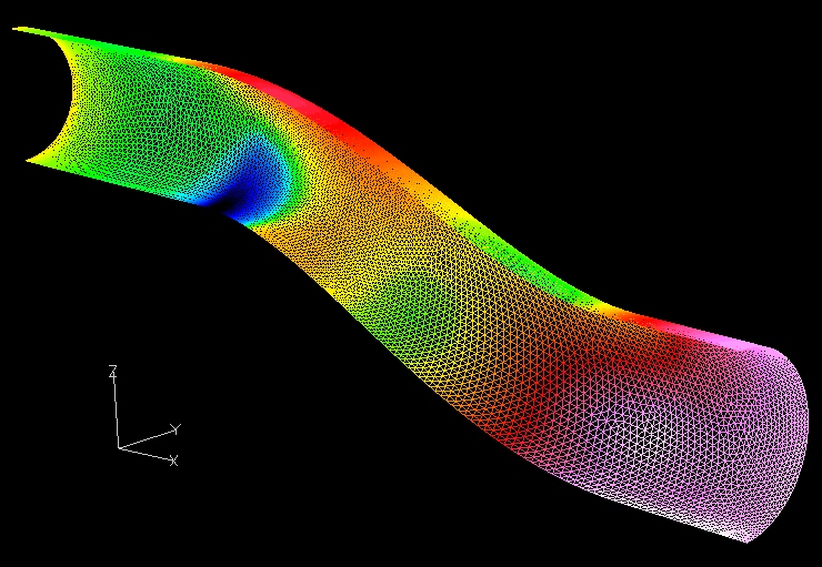
You will see contour plots of Mach number, total pressure, and
static pressure, velocity vectors and the grid.
The Mach number plot will look like so:
Further post-processing
Though not explained here, the following commerical software packages can be
used to open and view your CGD and CFL files:
-
Fieldview (if compiled with the special Boeing reader)
-
EnSight
If you know of additional packages, please let us know so that we may update
this list.